Sample 45701: Estimating the Standard Deviation of a Variable in a Finite Population
 |  |  |  |
Overview
The finite population standard deviation of a variable provides a measure of the amount of variation in the corresponding attribute of the study population’s members, thus helping to describe the distribution of a study variable. Whether your survey is measuring crop yields, adult alcohol consumption, or the body mass index (BMI) of school children, a small population standard deviation is indicative of uniformity in the population, while a large standard deviation is indicative of a more diverse population.
Suppose you have data that were sampled according to some complex survey design. The SURVEYMEANS procedure enables you to estimate sample totals, means, and ratios, as well as
the design-based variances of the estimated quantities, but it does not directly compute the standard deviation of a variable. However, because a standard deviation can be expressed
mathematically as a function of a total, you can easily estimate the finite population standard deviation
 of a
variable by using PROC SURVEYMEANS plus a little SAS programming.
of a
variable by using PROC SURVEYMEANS plus a little SAS programming.
Whenever you estimate a population parameter such as a mean or a standard deviation, you should also
report the precision of the estimate. The most commonly reported measure of precision is the variance (or its square root, the standard error). The survey analysis procedures
in SAS/STAT software currently provide three different variance estimation methods for complex survey designs: the Taylor series linearization method, the delete-one jackknife method,
and the balanced repeated replication (BRR) method. This example demonstrates how to use all three methods to estimate the variance
 .
.
Analysis
Suppose you want to estimate the standard deviation of a variable
 from a finite
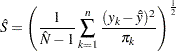
population by using data that were collected using some complex survey design. The finite population standard deviation of
is
from a finite
population by using data that were collected using some complex survey design. The finite population standard deviation of
is

|
(1) |
where  is
the total number of elements in the population,
is
the total number of elements in the population,
 is the
 th observation
of the variable ,
and
th observation
of the variable ,
and  is the
population mean of .
A sample-based statistic of
is
is the
population mean of .
A sample-based statistic of
is
|
(2) |
where  is an
estimator of the population total
,
is an
estimator of the population total
,
 is an estimator
of the population mean,
is an estimator
of the population mean,  is the number of elements in the sample, and
 is the probability
that element
is the probability
that element  is observed in the sample.
To estimate
 , you first estimate
both
, you first estimate
both  and
and
 with PROC SURVEYMEANS.
Next, you generate a variable (call it
with PROC SURVEYMEANS.
Next, you generate a variable (call it
 ) such that each
observation
) such that each
observation  is
equal to
is
equal to
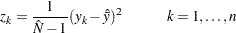
|
(3) |
Now you use PROC SURVEYMEANS to estimate the total of
. The square root
of the estimated weighted total of
is equal to
. Estimating
, the variance
of , requires
some additional SAS programming.
Using the Taylor Series Linearization Method to Estimate

To estimate  by using the
Taylor series linearization method, construct a variable
by using the
Taylor series linearization method, construct a variable
 , such that

|
(4) |
where is computed
as in equation (2). Use PROC SURVEYMEANS to estimate the total (and the variance of the total) of
. The total that
is computed by PROC SURVEYMEANS is of no interest, but the variance of the total is equal to
 , the variance
of the estimate
(Särndal, Swensson, and Wretman 1992
, chap. 5.5).
, the variance
of the estimate
(Särndal, Swensson, and Wretman 1992
, chap. 5.5).
The following steps summarize how you estimate
, the finite
population standard deviation of a variable
, and
, the variance
of the finite population standard deviation estimator (using the Taylor series linearization method):
-
Use PROC SURVEYMEANS to estimate the sample mean of the variable
, and
save the estimated mean. PROC SURVEYMEANS also computes the sum of the sampling weights, which is the value of
 in the
analysis. Save that value also; it is used in the construction of
.
in the
analysis. Save that value also; it is used in the construction of
. -
Using the sample mean from step 1, construct the variable
as
in equation (3). -
Use PROC SURVEYMEANS to estimate the weighted total of the variable
. Save
the estimated total, which is the estimate of the population variance
( ).
Take the square root of the weighted total. Save the result, which is the estimate of the finite population standard deviation.
).
Take the square root of the weighted total. Save the result, which is the estimate of the finite population standard deviation. -
Construct the variable
as in
equation (4). -
Use PROC SURVEYMEANS to estimate the weighted total (and the variance of the total) of the variable
. The
estimated variance of this total obtained from PROC SURVEYMEANS is an estimator of the variance of
.
Example
Ice Cream Study Data Set
This example uses the IceCreamStudy data set from the example "Stratified Cluster Sample Design" in the chapter "The SURVEYMEANS Procedure" of the SAS/STAT User's Guide.
The study population is a junior high school with a total of 4,000 students in grades 7, 8, and 9. In the
original example, researchers want to know how much these students spend weekly for ice cream, on the average, and what percentage of students spend at least $10 weekly for ice
cream. This example measures the variability of the students’ expenditures by estimating
 , the
variance of the variable that contains the students’ expenditures.
, the
variance of the variable that contains the students’ expenditures.
Suppose that every student belongs to a study group and that study groups are formed within each grade level. Each study group contains between two and four students. Table 1 shows the total number of study groups and the total number of students for each grade.
|
Grade |
Number of Study Groups |
Number of Students |
|---|---|---|
|
7 |
608 |
1,824 |
|
8 |
252 |
1,025 |
|
9 |
403 |
1,151 |
It is quicker and more convenient to collect data from students in the same study group than to collect data from students individually. Therefore, this study uses a stratified clustered sample design. The primary sampling units are study groups. The list of all study groups in the school is stratified by grade level. From each grade level, a sample of study groups is randomly selected, and all students in each selected study group are interviewed. The sample consists of eight study groups from the 7th grade, three groups from the 8th grade, and five groups from the 9th grade.
The SAS data set IceCreamStudy saves the responses of the selected students:
data IceCreamStudy;
   input Grade StudyGroup Spending Weight @@;
   datalines;
7  34  7 76.0   7  34  7 76.0  7 412  4 76.0  9  27 14 80.6
7  34  2 76.0   9 230 15 80.6  9  27 15 80.6  7 501  2 76.0
9 230  8 80.6   9 230  7 80.6  7 501  3 76.0  8  59 20 84.0
7 403  4 76.0   7 403 11 76.0  8  59 13 84.0  8  59 17 84.0
8 143 12 84.0   8 143 16 84.0  8  59 18 84.0  9 235  9 80.6
8 143 10 84.0   9 312  8 80.6  9 235  6 80.6  9 235 11 80.6
9 312 10 80.6   7 321  6 76.0  8 156 19 84.0  8 156 14 84.0
7 321  3 76.0   7 321 12 76.0  7 489  2 76.0  7 489  9 76.0
7  78  1 76.0   7  78 10 76.0  7 489  2 76.0  7 156  1 76.0
7  78  6 76.0   7 412  6 76.0  7 156  2 76.0  9 301  8 80.6
;
Table 2 identifies the variables contained in the data set IceCreamStudy.
|
Variable |
Description |
|---|---|
|
Grade |
Student’s grade (strata) |
|
StudyGroup |
Student’s study group (PSU) |
|
Spending |
Student’s expenditure per week for ice cream, in dollars |
|
Weight |
Sampling weights |
The SAS data set StudyGroup is created to provide PROC SURVEYMEANS with the sample design information shown in Table 1. The variable Grade identifies the strata, and the variable _TOTAL_ contains the total number of study groups in each stratum.
data StudyGroups;
   input Grade _total_;
   datalines;
7 608
8 252
9 403
;
Step 1: Compute
and
Use PROC SURVEYMEANS to obtain an estimate of the sample mean. Specify the MEAN and STACKING options in the PROC SURVEYMEANS statement. The STACKING option causes the procedure to create an output
data set with a single observation. This table structure makes it easy in later steps to identify the saved estimates and to assign their values to macro variables. The WEIGHT statement specifies that
the variable Weight contain the sampling weights. The STRATA statement specifies that the variable Grade identifies strata membership. The
CLUSTER statement specifies that the variable StudyGroup identifies cluster (or PSU) membership. The ODS OUTPUT statement requests output data sets for the statistics
and data summary tables, to be named Statistics and Summary, respectively. The sample mean is stored in the data set
Statistics. The data set Summary contains the sum of the sampling weights, the number of strata, and the number of clusters. The sum of the
sampling weights is needed to compute ;
the number of strata and the number of clusters are used later to compute confidence limits for
.
proc surveymeans data=IceCreamStudy mean stacking ;
   weight Weight;
   strata Grade;
   cluster StudyGroup;
   var Spending;
   ods output Statistics = Statistics
              Summary = Summary;
run;
The following DATA step saves the sample mean of the variable Spending in a macro variable named Spending_Mean:
data _null_;
   set Statistics;
   call symput("Spending_Mean",Spending_Mean);
run;
The next DATA step saves the sum of the sampling weights in a macro variable named N, the number of strata in a macro variable named H, and the number of clusters in a macro variable named C:
data Summary;
   set Summary;
   if Label1="Sum of Weights" then call symput("N",cValue1);
   if Label1="Number of Strata" then call symput("H",cValue1);
   if Label1="Number of Clusters" then call symput("C",cValue1);
run;
Step 2: Construct the Variable
Construct the variable in a DATA
step by using the macro variables Spending_Mean and N:
data Working;
   set IceCreamStudy;
   z=(1/(&N-1))*(Spending-&Spending_Mean)**2;
run;
Step 3: Estimate the Total of
and Take the
Square Root of the Total
Use PROC SURVEYMEANS to estimate the weighted total of the variable
. Specify the SUM and STACKING options
in the PROC SURVEYMEANS statement. The ODS OUTPUT statement saves the statistics table to a data set named Result.
proc surveymeans data = Working sum stacking;
   weight Weight;
   var z;
   ods output Statistics = Result;
run;
The following DATA step retrieves the estimated total of
and stores it in a macro
variable named Variance. The total of
is equal to
. Take the square root of the
estimated total and store it in a macro variable named StdDev. The square root of the estimated total is the finite population standard deviation
.
data Result;
   set Result;
   StdDev=sqrt(z_Sum);
   call symput("Variance",z_Sum);
   call symput("StdDev",StdDev);
run;
Step 4: Construct the Variable
Construct the variable by using
the macro variables Spending_Mean, N, Variance, and StdDev.
data Taylor;
   set IceCreamStudy;
   u=((Spending-&Spending_Mean)**2 - &Variance)/(2*&StdDev*(&N-1));
run;
Step 5: Estimate the Total of
Use PROC SURVEYMEANS to estimate the total of the variable
. Specify the SUM, VARSUM, TOTAL=,
and STACKING options in the PROC SURVEYMEANS statement. The VARSUM option computes the variance of the total. In this step, the computation of interest is the variance of the estimated total rather than
the total itself. Therefore, the sampling design must be appropriately represented in the SURVEYMEANS procedure. The TOTAL= option enables the procedure to apply a finite population correction in the
variance computation. The STRATA statement specifies that the strata be identified by the variable Grade, and the CLUSTER statement specifies that cluster membership be
identified by the variable StudyGroup. The ODS OUTPUT statement saves the statistics table in a data set named Result.
proc surveymeans data = Taylor sum varsum stacking total=StudyGroups;
   strata Grade;
   cluster StudyGroup;
   weight Weight;
   var u;
   ods output Statistics = Result;
run;
The following DATA step creates the variable Estimate in the data set Result and assigns it the value of
that is
stored in the macro variable StdDev. The
 confidence
limits are computed, and the data set Result is prepared for printing.
confidence
limits are computed, and the data set Result is prepared for printing.
%let df=%eval(&C - &H);

data Result;
   set Result(rename=(u_VarSum=Variance
                      u_StdDev=StdErr));
   Estimate=&StdDev;
   LowerCL= Estimate + StdErr*TINV(.025,&df);
   UpperCL= Estimate + StdErr*TINV(.975,&df);
   label Estimate=Population Standard Deviation Estimate
         Variance=Variance of Estimate
         StdErr=Standard Error of Estimate
         LowerCL=Lower Confidence Limit
         UpperCL=Upper Confidence Limit;
   Variable='Spending';
run;
Use PROC PRINT to print the contents of the data set Result:
title 'Parameter Estimates';

proc print data=Result label noobs;
   var Variable Estimate Variance StdErr LowerCL UpperCL;
run;

title ;
Output 1 displays the results. The estimate of the population standard deviation of the variable Spending is 5.33. The variance of the estimate is 0.245. The standard error of the estimate is 0.49, and the estimated lower and upper 95% confidence limits are 4.27 and 6.40, respectively.
| Parameter Estimates |
| Variable | Population Standard Deviation Estimate |
Variance of Estimate | Standard Error of Estimate |
Lower Confidence Limit |
Upper Confidence Limit |
|---|---|---|---|---|---|
| Spending | 5.33483 | 0.244809 | 0.494782 | 4.26592 | 6.40374 |
Using the Delete-One Jackknife Method to Estimate
The delete-one jackknife resampling method of variance estimation deletes one primary sampling unit (PSU) at a time from the full sample to create
 replicates,
where is the total number
of PSUs. In each replicate, the sample weights of the remaining PSUs are modified by the jackknife coefficient
replicates,
where is the total number
of PSUs. In each replicate, the sample weights of the remaining PSUs are modified by the jackknife coefficient
 . The modified
weights are called replicate weights.
. The modified
weights are called replicate weights.
If
 is the estimate of
obtained using only the
data and the replicate weights from the
is the estimate of
obtained using only the
data and the replicate weights from the  th
replicate, the jackknife variance estimate
is
th
replicate, the jackknife variance estimate
is
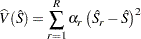
|
(5) |
with  degrees of
freedom, where
is the jackknife coefficient for the
th replicate,
is the number of
replicates, and
degrees of
freedom, where
is the jackknife coefficient for the
th replicate,
is the number of
replicates, and  is
the number of strata (or
is
the number of strata (or  when there is no stratification). See the section Jackknife Method
in the chapter "The SURVEYMEANS Procedure" of the SAS/STAT User's Guide for more details.
when there is no stratification). See the section Jackknife Method
in the chapter "The SURVEYMEANS Procedure" of the SAS/STAT User's Guide for more details.
Recall that when you construct
, you use estimates of
and
that are computed by using the full sample. However, the jackknife variance estimator requires that the be computed from the th replicate. Thus, the jackknife estimate of the variance of the total of is not equal to the jackknife estimate of the variance of .
The following steps summarize how you estimate , the finite population standard deviation of a variable , and
, the variance of the finite population standard deviation estimator (using the delete-one jackknife method):
-
Use PROC SURVEYMEANS to estimate the sample mean
and the sum of the weights
for the full sample. Save both estimates as they are used in the construction of
. -
Construct
as in equation (3), using the full-sample estimates of
and
obtained in step 1. -
Use PROC SURVEYMEANS to estimate the weighted total of the variable
.
Take the square root of the total, and save the result, which is the full-sample estimate of the population standard deviation
().
When you estimate the total, specify the VARMETHOD=JACKKNIFE option and the OUTWEIGHTS= and OUTJKCOEFS= method-options in the PROC SURVEYMEANS statement. Both
the OUTWEIGHTS= and OUTJKCOEFS= data sets are used in later steps. -
For each replicate, use PROC SURVEYMEANS to compute the sample mean
 and
the sum of the weights
and
the sum of the weights
 by using
only the data and replicate weights for the
th replicate.
Save the estimates for later use.
by using
only the data and replicate weights for the
th replicate.
Save the estimates for later use. -
For each replicate, using the estimates for
and
that were obtained in step 4, construct the variable
such that

(6) -
Use PROC SURVEYMEANS to estimate the weighted total of
by replicate.
Take the square root of each estimated total, and save the results for later use. The square root of the estimated weighted total of
 is
equal to
is
equal to  for the th
replicate.
for the th
replicate. -
Construct a variable (call it
) by using the
estimates
from step 6, the jackknife coefficients, and the full-sample estimate
from
step 3 such that 
-
Use PROC SURVEYMEANS to estimate the unweighted total of the variable
from step 7. The estimated unweighted total of
is
,
the delete-one jackknife estimate of the variance of
.
Example
This example uses the same IceCreamStudy data set that was described in the section Ice Cream Study Data Set and
reproduces the steps described in the section Using the Delete-One Jackknife Method to Estimate
. Steps 1 and 2 are identical to the first two steps in the previous example but are repeated here for completeness.
Step 1: Compute
and for the Full
Sample
Use PROC SURVEYMEANS to obtain an estimate of the sample mean. Specify the MEAN and STACKING options in the PROC SURVEYMEANS statement. The WEIGHT statement specifies that the variable Weight contain the sampling weights. The STRATA statement specifies that the variable Grade identifies strata membership. The CLUSTER statement specifies that the variable StudyGroup identifies cluster (or PSU) membership. The ODS OUTPUT statement creates output data sets for the statistics and data summary tables, to be named Statistics and Summary, respectively. The sample mean is stored in the data set Statistics. The data set Summary contains the sum of the sampling weights and the number of strata.
proc surveymeans data=IceCreamStudy mean stacking ;
   weight Weight;
   strata Grade;
   cluster StudyGroup;
   var Spending;
   ods output Statistics = Statistics
              Summary = Summary;
run;
The following DATA step saves the sample mean of the variable Spending in a macro variable named Spending_Mean:
data _null_;
   set Statistics;
   call symput("Spending_Mean",Spending_Mean);
run;
The next DATA step saves the sum of the sampling weights in a macro variable named N and the number of strata in a macro variable named H:
data Summary;
   set Summary;
   if Label1="Sum of Weights" then call symput("N",cValue1);
   if Label1="Number of Strata" then call symput("H",cValue1);
run;
Step 2: Construct the Variable
Using the Full-Sample Estimates of
and
Construct the variable
in a DATA step using the macro variables Spending_Mean and N:
data Working;
   set IceCreamStudy;
   Z=(1/(&N-1))*(Spending-&Spending_Mean)**2;
run;
Step 3: Estimate the Total of
for the
Full Sample
Use PROC SURVEYMEANS to estimate the weighted total of the variable
. Specify the SUM and STACKING
options in the PROC SURVEYMEANS statement. Also specify the VARMETHOD=JACKKNIFE option with the OUTJKCOEFS= and OUTWEIGHTS= method-options. The OUTJKCOEFS= method-option saves the jackknife
coefficients in a SAS data set named Jkcoefs. The OUTWEIGHTS= method-option saves the replicate weights in a SAS data set named Jkweights.
In this step you must fully specify the sampling design so that the jackknife coefficients and replicate weights are computed correctly. The STRATA statement specifies that the strata be identified by the variable Grade. The CLUSTER statement specifies that the PSUs be identified by the variable StudyGroup. The WEIGHT statement specifies that the full-sample sampling weights be contained in the variable Weight. The ODS OUTPUT statement saves the statistics table to a data set named Result and the variance estimation table to a data set named VarianceEstimation.
proc surveymeans data=Working sum stacking
                 varmethod=JACKKNIFE(outjkcoefs=Jkcoefs outweights=Jkweights);
   strata Grade /list;
   cluster StudyGroup;
   weight Weight;
   var z;
   ods output Statistics = Result
              VarianceEstimation=VarianceEstimation;
run;
You can see from the "Variance Estimation" table in Output 2 that there are 16 replicates.
| Data Summary | |
|---|---|
| Number of Strata | 3 |
| Number of Clusters | 16 |
| Number of Observations | 40 |
| Sum of Weights | 3162.6 |
| Variance Estimation | |
|---|---|
| Method | Jackknife |
| Number of Replicates | 16 |
The next DATA step retrieves the number of replicates and stores the value in a macro variable named R:
data _null_;
   set VarianceEstimation;
   where label1="Number of Replicates";
   call symput("R",cvalue1);
run;

%let R=%eval(&R);
The data set Jkcoefs has 16 observations, one for each replicate. The
th observation
contains the jackknife coefficient for the
th replicate.
The data set Jkweights contains the original variables from the IceCreamStudy data set and 16 new variables named
RepWgt_1 through RepWgt_16; there are
 observations.
The following DATA step retrieves the estimated total of the variable
, takes the
square root of the estimated total, and stores it in a macro variable named StdDev. The square root of the weighted total of the variable
is
.
data _null_;
   set Result;
   StdDev=sqrt(Z_Sum);
   call symput("StdDev",StdDev);
run;
Step 4: Compute
and for Replicate
Samples
Before computing and
, use the following DATA step to
convert the data set Jkweights from wide form to long form; doing so enables you to use BY-group processing with PROC SURVEYMEANS.
data Long(drop= RepWt_1 - RepWt_&R Z);
  set Jkweights;
  array num (*) RepWt_1 - RepWt_&R;
  do replicate=1 to dim(num);
    Jkweight=num(replicate);
   output;
  end;
run;
The data set Long has
 observations.
There are 16 copies of the original variables from the IceCreamStudy data set stacked on top of each other, and each copy is identified by the variable
Replicate. Instead of the 16 replicate weight variables, RepWgt_1 through RepWgt_16, there is
now one variable, Jkweight, which is constructed by stacking the variables RepWgt_1 through RepWgt_16
on top of each other. Thus, the first 40 observations contain a copy of the original variables, the contents of RepWgt_1, and the variable
Replicate has a value of 1. The second 40 observations contain a copy of the original variables, the contents of RepWgt_2,
and the variable Replicate has a value of 2. The remaining observations are constructed and identified similarly.
observations.
There are 16 copies of the original variables from the IceCreamStudy data set stacked on top of each other, and each copy is identified by the variable
Replicate. Instead of the 16 replicate weight variables, RepWgt_1 through RepWgt_16, there is
now one variable, Jkweight, which is constructed by stacking the variables RepWgt_1 through RepWgt_16
on top of each other. Thus, the first 40 observations contain a copy of the original variables, the contents of RepWgt_1, and the variable
Replicate has a value of 1. The second 40 observations contain a copy of the original variables, the contents of RepWgt_2,
and the variable Replicate has a value of 2. The remaining observations are constructed and identified similarly.
Next, sort the data set Long by Replicate:
proc sort data=Long out=Long;
   by Replicate;
run;
Use PROC SURVEYMEANS to estimate the mean of Spending by Replicate. Doing so produces the estimates of
 and
and  for each replicate. The WEIGHT statement specifies that the sampling weights be contained in the variable Jkweight. The ODS OUTPUT statement saves
the sample means ()
in a SAS data set named JKMeans and the sums of the replicate weights
() in a data
set named JKN. By default, the means are stored in a variable named Mean and the sums of the replicate weights are
stored in a variable named N.
for each replicate. The WEIGHT statement specifies that the sampling weights be contained in the variable Jkweight. The ODS OUTPUT statement saves
the sample means ()
in a SAS data set named JKMeans and the sums of the replicate weights
() in a data
set named JKN. By default, the means are stored in a variable named Mean and the sums of the replicate weights are
stored in a variable named N.
proc surveymeans data=Long mean;
   weight Jkweight;
   var Spending;
   by Replicate;
   ods output Statistics = JKMeans(keep=Replicate Mean)
              Summary = JKN;
run;
Step 5: Construct the Variable
for
Replicate Samples
Before you can construct the variable
for the replicate samples, you must merge the data sets JKMeans and JKN with Long, by Replicate:
proc sort data=JKMeans out=JKMeans;
   by Replicate;
run;
data JKN(keep=N replicate );
   set JKN(rename=(nvalue1=N));
   where Label1="Sum of Weights";
run;
proc sort data=JKN out=JKN;
   by Replicate;
run;
data Long;
   merge Long JKN JKMeans;
   by Replicate;
run;
Now construct the variable
using the merged data set.
data Long;
   set Long;
   z=(1/(N-1))*(Spending-Mean)**2;
run;
Step 6: Estimate the Total of
for Replicate
Samples
Use PROC SURVEYMEANS to estimate the total of the variable
by Replicate. The WEIGHT statement specifies that the sampling weights be contained in the variable Jkweight. You do not
need to specify the STRATA and CLUSTER statements. The ODS OUTPUT statement saves the estimated totals in the variable JKEstimate in a SAS data set named
Statistics. The estimated totals are the estimates
 for each replicate.
proc surveymeans data=Long sum stacking;
   weight Jkweight;
   var z;
   by Replicate;
   ods output Statistics=Statistics(rename=(Z_Sum=JKEstimate));
run;
Take the positive square roots of the estimated totals. The results are the estimates
for
each replicate.
data Statistics;
   set Statistics(drop=Z_StdDEV z);
   JKEstimate=sqrt(JKEstimate);
run;
Step 7: Construct the Variable
Before you can construct the variable
, you must sort and merge,
by Replicate, the data sets Statistics and Jkcoefs:
proc sort data=Statistics out=Statistics;
   by Replicate;
run;
proc sort data=Jkcoefs out=Jkcoefs;
   by Replicate;
run;
data Statistics;
   merge Statistics Jkcoefs;
   by Replicate;
run;
The data set Statistics now contains the jackknife coefficients
in the
variable JKcoefficients and the estimates
in
the variable JKEstimate. Construct the variable
by using
these variables and the full-sample estimate
that is
saved in the macro variable StdDev.
data Statistics;
   set Statistics;
   u=JKcoefficient*(JKEstimate-&StdDev)**2;
run;
Step 8: Estimate the Total of
Use PROC SURVEYMEANS to compute the unweighted total of
. Specify the
SUM option in the PROC SURVEYMEANS statement. The ODS OUTPUT statement saves the total in a variable named Variance in a SAS data set named Result.
proc surveymeans data=Statistics sum;
   var u;
   ods output Statistics=Result(rename=(sum=Variance));
run;
The following DATA step computes the standard error of the estimate and the upper and lower 95% confidence limits. In this example, the confidence limits are computed using a
 distribution
with
distribution
with  degrees
of freedom. The variable Estimate is generated and assigned the estimated value of
that is
stored in the macro variable StdDev. Labels are created for the existing variables, a new variable Variable is generated,
and its value is specified to be the name of the variable that is being analyzed (Spending).
degrees
of freedom. The variable Estimate is generated and assigned the estimated value of
that is
stored in the macro variable StdDev. Labels are created for the existing variables, a new variable Variable is generated,
and its value is specified to be the name of the variable that is being analyzed (Spending).
%let df=%eval(&R-&H);

data Result;
   set Result;
   StdErr=sqrt(Variance);
   Estimate=&StdDev;
   UpperCL=Estimate + StdErr*TINV(.975,&df);
   LowerCL=Estimate + StdErr*TINV(.025,&df);
   label Estimate=Population Standard Deviation Estimate
         Variance=Variance of Estimate
         StdErr=Standard Error of Estimate
         LowerCL=Lower Confidence Limit
         UpperCL=Upper Confidence Limit;
   Variable='Spending';
run;
Use the PRINT procedure to print the contents of the data set Result:
title 'Parameter Estimates';

proc print data=Result label noobs;
   var Variable Estimate Variance StdErr LowerCL UpperCL;
run;

title ;
Output 3 displays the results. The estimate of the population standard deviation for the variable Spending is 5.33. The variance of the estimate is 0.27, and the standard error of the estimate is 0.52. The estimated lower and upper 95% confidence limits are 4.21 and 6.46, respectively.
| Parameter Estimates |
| Variable | Population Standard Deviation Estimate |
Variance of Estimate | Standard Error of Estimate |
Lower Confidence Limit |
Upper Confidence Limit |
|---|---|---|---|---|---|
| Spending | 5.33483 | 0.271465 | 0.52102 | 4.20923 | 6.46043 |
Using the BRR Method to Estimate
The BRR method requires that the full sample be drawn by using a stratified sample design with two PSUs per stratum. If
is the total number of strata,
the total number of replicates is
the smallest multiple of four that is greater than
. Each replicate is obtained
by deleting one PSU per stratum according to the corresponding Hadamard matrix and adjusting the original weights for the remaining PSUs. The new weights are called replicate weights.
If is the estimate of
obtained by using only the data
and the replicate weights from the th
replicate, the BRR variance estimate
is
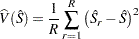
|
(7) |
with
degrees of freedom. See the section Balanced Repeated
Replication (BRR) Method in the chapter "The SURVEYMEANS Procedure" of the SAS/STAT User's Guide for more details.
Recall that when you construct
,
you use estimates of
and that are
computed by using the full sample. However, the BRR variance estimator requires that the
be
computed from the th
replicate. Thus, the BRR estimate of the variance of the total of
is not equal to
the BRR estimate of the variance of
.
The following steps summarize how you estimate
, the finite population
standard deviation of a variable
,
and , the
variance of the finite population standard deviation estimator (using the BRR method):
-
Use PROC SURVEYMEANS to estimate the sample mean
and
the sum of the weights
for
the full sample. Save both estimates for later use: they are used in the construction of
.
Also save the number of strata
for later use.
-
Construct
as in equation (3) by using the full-sample estimates of
and
obtained
in step 1. -
Use PROC SURVEYMEANS to estimate the weighted total of the variable
, take
the square root of the estimated total, and save the result. The square root of the estimated total is the full-sample estimate of the population standard deviation
().
When you estimate the total, specify the VARMETHOD=BRR option and the OUTWEIGHTS= method-option in the PROC SURVEYMEANS statement. The OUTWEIGHTS= SAS data set is used in
later steps. Also save the number of replicates
for later use.
-
For each replicate, use PROC SURVEYMEANS to estimate the sample mean
and
the sum of the weights
by using
only the data and replicate weights for the
th replicate.
Save the estimates for later use. -
For each replicate, using the estimates for
and
that
were obtained in step 4, construct the variable
such that
(8) -
Use PROC SURVEYMEANS to estimate the weighted total of
by replicate,
take the positive square root of each estimated total, and save the results for later use. The square root of the estimated weighted total of
is equal
to for the
th replicate. -
Construct a variable (call it
) by using
the estimates
from step 6, the number of replicates
, and
the full-sample estimate
from
step 3 such that 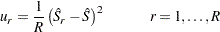
-
Use PROC SURVEYMEANS to estimate the unweighted total of the variable
from step 7. The estimated unweighted total of
is
,
the BRR estimate of the variance of
.
Example
This example uses the MUNIsurvey data set from the section Variance Estimation Using Replication Methods in the chapter "The SURVEYMEANS Procedure" of the SAS/STAT User's Guide. The data are not shown here, but a SAS program that generates the data is included in the sample SAS code that you can download for this example.
In the original example, the San Francisco Municipal Railway (MUNI) conducted a survey to estimate the average waiting time for MUNI subway system’s passengers. This example estimates the standard deviation of the passengers’ waiting time.
The study uses a stratified cluster sample design. Each MUNI subway line is a stratum. The subway lines included in the study are 'J-Church,' 'K-Ingleside,' 'L-Taraval,' 'M-Ocean View,' 'N-Judah,' and the street car 'F-Market & Wharves.' The MUNI vehicles in service for these lines during a day are the primary sampling units. Within each stratum, two vehicles (PSUs) are randomly selected. Then the waiting times of passengers for a selected MUNI vehicle are collected.
The collected data are saved in the SAS data set MUNIsurvey. Table 3 identifies the variables contained in the data set.
|
Variable |
Description |
|---|---|
|
Line |
The MUNI line that a passenger is riding (strata) |
|
Vehicle |
The vehicle that a passenger is boarding (PSU) |
|
Waittime |
The time (in minutes) that a passenger waited |
|
Weight |
Sampling weights |
Step 1: Compute
and for the
Full Sample
Use PROC SURVEYMEANS to obtain estimates of the sample mean
() and the sum of the
sampling weights () for
the full sample. Specify the MEAN and STACKING options in the PROC SURVEYMEANS statement. The WEIGHT statement specifies that the sampling weights be contained in the variable
Weight.
The STRATA statement specifies that the strata be identified by the variable Line. The CLUSTER statement specifies that the PSUs be identified by the variable
Vehicle. The ODS OUTPUT statement produces output data sets for the statistics and data summary tables, to be named Statistics and
Summary, respectively. The sample mean is stored in the data set Statistics. The sum of the sampling weights and the number of strata
are stored in the data set Summary.
proc surveymeans data=MUNIsurvey mean stacking ;
   weight Weight;
   strata Line;
   cluster Vehicle;
   var Waittime;
   ods output Statistics = Statistics
              Summary = Summary;
run;
The following DATA step saves the sample mean
() of the
variable Waittime in a macro variable named Waittime_Mean:
data _null_;
   set Statistics;
   call symput("Waittime_Mean",Waittime_Mean);
run;
The next DATA step saves the sum of the sampling weights in a macro variable named N and the number of strata in a macro variable named H:
data Summary;
   set Summary;
   if Label1="Sum of Weights" then call symput("N",cValue1);
   if Label1="Number of Strata" then call symput("H",cValue1);
run;
Step 2: Construct the Variable
Using the Full-Sample Estimates of
and
Construct the variable
in a DATA step by using the macro variables Waittime_Mean and N:
data Working;
   set MUNIsurvey;
   Z=(1/(&N-1))*(Waittime-&Waittime_Mean)**2;
run;
Step 3: Estimate the Total of
for the Full Sample
Use PROC SURVEYMEANS to estimate the total of the variable
. Specify the SUM and
STACKING options in the PROC SURVEYMEANS statement. Also specify the VARMETHOD=BRR OUTWEIGHTS= method-options. The OUTWEIGHTS= method-option saves the replicate weights in a SAS data set
named BRRweights.
In this step you must fully specify the sampling design so that the replicate weights are computed correctly. The STRATA statement specifies that the strata be identified by the variable Line. The CLUSTER statement specifies that the PSUs be identified by the variable Vehicle. The WEIGHT statement specifies that the full-sample sampling weights be contained in the variable Weight. The ODS OUTPUT statement saves the statistics table to a data set named Estimate and the variance estimation table to a data set named VarianceEstimation.
proc surveymeans data=Working sum stacking
                 varmethod=brr(outweights=BRRweights);
   strata Line;
   cluster Vehicle;
   weight Weight;
   var z;
   ods output Statistics = Estimate
              VarianceEstimation=VarianceEstimation;
run;
| Data Summary | |
|---|---|
| Number of Strata | 6 |
| Number of Clusters | 12 |
| Number of Observations | 1937 |
| Sum of Weights | 143040 |
| Variance Estimation | |
|---|---|
| Method | BRR |
| Number of Replicates | 8 |
There are  observations and
  replicates. The data set BRRweights contains the original variables from the Munisurvey data set and eight new variables named
RepWgt_1 through RepWgt_8.
replicates. The data set BRRweights contains the original variables from the Munisurvey data set and eight new variables named
RepWgt_1 through RepWgt_8.
The following DATA step retrieves the estimated total of the variable
,
takes the square root of the total, and stores the result in a macro variable named StdDev. The square root of the total of the variable
is
equal to .
data _null_;
   set Estimate;
   StdDev=sqrt(Z_Sum);
   call symput("StdDev",StdDev);
run;
The next DATA step retrieves the number of replicates and stores the value in a macro variable named R:
data _null_;
   set VarianceEstimation;
   where label1="Number of Replicates";
   call symput("R",cvalue1);
run;

%let R=%eval(&R);
Step 4: Compute
and
for Replicate Samples
Before computing
and , use the following
DATA step to convert the data set BRRweights from wide form to long form; doing so enables you to use BY-group processing with PROC SURVEYMEANS.
data Long(drop= RepWt_1 - RepWt_&R Z);
  set BRRweights;
  array num (*) RepWt_1 - RepWt_&R;
  do replicate=1 to dim(num);
    BRRweight=num(replicate);
   output;
  end;
run;
The data set Long has
 observations. There are eight copies of the original variables from the Munisurvey data set stacked on top of each other, and each copy is identified
by the variable Replicate. Instead of the eight replicate weight variables, RepWgt_1 through
RepWgt_8, there is now one variable, BRRweight, which is constructed by stacking the variables
RepWgt_1 through RepWgt_8 on top of each other. Thus, the first 1,937 observations contain a copy of the original
variables and the contents of RepWgt_1, and the variable Replicate has a value of 1. The second 1,937 observations
contain a copy of the original variables and the contents of RepWgt_2, and the variable Replicate has a value of 2.
The remaining observations are constructed and identified similarly.
observations. There are eight copies of the original variables from the Munisurvey data set stacked on top of each other, and each copy is identified
by the variable Replicate. Instead of the eight replicate weight variables, RepWgt_1 through
RepWgt_8, there is now one variable, BRRweight, which is constructed by stacking the variables
RepWgt_1 through RepWgt_8 on top of each other. Thus, the first 1,937 observations contain a copy of the original
variables and the contents of RepWgt_1, and the variable Replicate has a value of 1. The second 1,937 observations
contain a copy of the original variables and the contents of RepWgt_2, and the variable Replicate has a value of 2.
The remaining observations are constructed and identified similarly.
Next, sort the data set Long by Replicate:
proc sort data=Long out=Long;
   by Replicate;
run;
Use PROC SURVEYMEANS to estimate the mean of Waittime by Replicate. Doing so produces the estimates of
and
for each replicate. The WEIGHT statement specifies that the sampling weights be contained in the variable BRRweight. The ODS OUTPUT statement
saves the sample means in a SAS data set named BRRMeans and the sum of the replicate weights in a data set named BRRN.
proc surveymeans data=Long mean;
   weight BRRweight;
   var Waittime;
   by Replicate;
   ods output Statistics = BRRMeans(keep=Replicate Mean)
              Summary = BRRN;
run;
Step 5: Construct the Variable
Before you can construct the variable
, you must merge the data
sets BRRMeans and BRRN with Long by Replicate:
proc sort data=BRRMeans out=BRRMeans;
   by Replicate;
run;
data BRRN(keep=N replicate );
   set BRRN(rename=(nvalue1=N));
   where Label1="Sum of Weights";
run;
proc sort data=BRRN out=BRRN;
   by Replicate;
run;
data Long;
   merge Long BRRN BRRMeans;
   by Replicate;
run;
Now construct the variable
using the merged data set:
data Long;
   set Long;
   z=(1/(N-1))*(Waittime-Mean)**2;
run;
Step 6: Estimate the Total of
for the
Replicate Samples
Use PROC SURVEYMEANS to estimate the total of the variable
by
Replicate. The WEIGHT statement specifies that the sampling weights be contained in the variable BRRweight. You do not need to specify the
STRATA and CLUSTER statements. The ODS OUTPUT statement saves the estimated totals in the variable BRREstimate in a SAS data set named Statistics.
The estimated totals are the estimates  for each replicate.
proc surveymeans data=Long sum stacking;
   weight BRRweight;
   var z;
   by Replicate;
   ods output Statistics=Statistics(rename=(Z_Sum=BRREstimate));
run;
Take the square root of each estimated total. The results are the estimates
for each
replicate.
data Statistics;
   set Statistics(drop= Z_StdDEV z);
   BRREstimate=sqrt(BRREstimate);
run;
Step 7: Construct the Variable
data Statistics;
   set Statistics;
   u=(1/&R)*(BRREstimate-&StdDev)**2;
run;
Step 8: Estimate the Total of
Use PROC SURVEYMEANS to compute the unweighted total of
. Specify the SUM option in the
PROC SURVEYMEANS statement. The ODS OUTPUT statement saves the total in a variable named Variance in a SAS data set named Result.
proc surveymeans data=Statistics sum;
   var u;
   ods output Statistics=Result(rename=(sum=Variance));
run;
The following DATA step computes the standard error of the estimate and the upper and lower 95% confidence limits. The confidence limits for this example are
computed by using a
distribution with H=6 degrees of freedom. The variable Estimate is generated and assigned the estimated value of
,
which is stored in the macro variable StdDev. The data set is also prepared for printing.
data Result;
   set Result;
   StdErr=sqrt(Variance);
   Estimate=&StdDev;
   UpperCL=Estimate + StdErr*TINV(.975,&H);
   LowerCL=Estimate + StdErr*TINV(.025,&H);
   Variable='Waittime';
   label Estimate=Population Standard Deviation Estimate
         Variance=Variance of Estimate
         StdErr=Standard Error of Estimate
         LowerCL=Lower Confidence Limit
         UpperCL=Upper Confidence Limit;
run;
Use the PRINT procedure to print the contents of the data set Result:
title 'Parameter Estimates';

proc print data=Result label noobs;
   var Variable Estimate Variance StdErr LowerCL UpperCL;
run;

title ;
Output 5 displays the results. The estimate of the population standard deviation for the variable Waittime is 4.24. The variance of the estimate is 0.03, and the standard error of the estimate is 0.17. The estimated lower and upper 95% confidence limits are 3.82 and 4.67, respectively.
| Parameter Estimates |
| Variable | Population Standard Deviation Estimate |
Variance of Estimate | Standard Error of Estimate |
Lower Confidence Limit |
Upper Confidence Limit |
|---|---|---|---|---|---|
| Waittime | 4.24495 | 0.029935 | 0.17302 | 3.82159 | 4.66831 |
References
-
Särndal, C. E., Swensson, B., and Wretman, J. (1992), Model Assisted Survey Sampling, New York: Springer-Verlag.
These sample files and code examples are provided by SAS Institute Inc. "as is" without warranty of any kind, either express or implied, including but not limited to the implied warranties of merchantability and fitness for a particular purpose. Recipients acknowledge and agree that SAS Institute shall not be liable for any damages whatsoever arising out of their use of this material. In addition, SAS Institute will provide no support for the materials contained herein.
data IceCreamStudy;
   input Grade StudyGroup Spending Weight @@;
   datalines;
7  34  7 76.0   7  34  7 76.0  7 412  4 76.0  9  27 14 80.6
7  34  2 76.0   9 230 15 80.6  9  27 15 80.6  7 501  2 76.0
9 230  8 80.6   9 230  7 80.6  7 501  3 76.0  8  59 20 84.0
7 403  4 76.0   7 403 11 76.0  8  59 13 84.0  8  59 17 84.0
8 143 12 84.0   8 143 16 84.0  8  59 18 84.0  9 235  9 80.6
8 143 10 84.0   9 312  8 80.6  9 235  6 80.6  9 235 11 80.6
9 312 10 80.6   7 321  6 76.0  8 156 19 84.0  8 156 14 84.0
7 321  3 76.0   7 321 12 76.0  7 489  2 76.0  7 489  9 76.0
7  78  1 76.0   7  78 10 76.0  7 489  2 76.0  7 156  1 76.0
7  78  6 76.0   7 412  6 76.0  7 156  2 76.0  9 301  8 80.6
;
data StudyGroups;
   input Grade _total_;
   datalines;
7 608
8 252
9 403
;
proc surveymeans data=IceCreamStudy mean stacking ;
   weight Weight;
   strata Grade;
   cluster StudyGroup;
   var Spending;
   ods output Statistics = Statistics
              Summary = Summary;
run;
data _null_;
   set Statistics;
   call symput("Spending_Mean",Spending_Mean);
run;
data Summary;
   set Summary;
   if Label1="Sum of Weights" then call symput("N",cValue1);
   if Label1="Number of Strata" then call symput("H",cValue1);
   if Label1="Number of Clusters" then call symput("C",cValue1);
run;

data Working;
   set IceCreamStudy;
   z=(1/(&N-1))*(Spending-&Spending_Mean)**2;
run;
proc surveymeans data = Working sum stacking;
   weight Weight;
   var z;
   ods output Statistics = Result;
run;
data Result;
   set Result;
   StdDev=sqrt(z_Sum);
   call symput("Variance",z_Sum);
   call symput("StdDev",StdDev);
run;
data Taylor;
   set IceCreamStudy;
   u=((Spending-&Spending_Mean)**2 - &Variance)/(2*&StdDev*(&N-1));
run;
proc surveymeans data = Taylor sum varsum stacking total=StudyGroups;
   strata Grade;
   cluster StudyGroup;
   weight Weight;
   var u;
   ods output Statistics = Result;
run;
%let df=%eval(&C - &H);

data Result;
   set Result(rename=(u_VarSum=Variance
                      u_StdDev=StdErr));
   Estimate=&StdDev;
   LowerCL= Estimate + StdErr*TINV(.025,&df);
   UpperCL= Estimate + StdErr*TINV(.975,&df);
   label Estimate=Population Standard Deviation Estimate
         Variance=Variance of Estimate
         StdErr=Standard Error of Estimate
         LowerCL=Lower Confidence Limit
         UpperCL=Upper Confidence Limit;
   Variable='Spending';
run;
title 'Parameter Estimates';

proc print data=Result label noobs;
   var Variable Estimate Variance StdErr LowerCL UpperCL;
run;

title ;
proc surveymeans data=IceCreamStudy mean stacking ;
   weight Weight;
   strata Grade;
   cluster StudyGroup;
   var Spending;
   ods output Statistics = Statistics
              Summary = Summary;
run;
data _null_;
   set Statistics;
   call symput("Spending_Mean",Spending_Mean);
run;
data Summary;
   set Summary;
   if Label1="Sum of Weights" then call symput("N",cValue1);
   if Label1="Number of Strata" then call symput("H",cValue1);
run;

data Working;
   set IceCreamStudy;
   Z=(1/(&N-1))*(Spending-&Spending_Mean)**2;
run;
proc surveymeans data=Working sum stacking
                 varmethod=JACKKNIFE(outjkcoefs=Jkcoefs outweights=Jkweights);
   strata Grade /list;
   cluster StudyGroup;
   weight Weight;
   var z;
   ods output Statistics = Result
              VarianceEstimation=VarianceEstimation;
run;
data _null_;
   set VarianceEstimation;
   where label1="Number of Replicates";
   call symput("R",cvalue1);
run;

%let R=%eval(&R);
data _null_;
   set Result;
   StdDev=sqrt(Z_Sum);
   call symput("StdDev",StdDev);
run;
data Long(drop= RepWt_1 - RepWt_&R Z);
  set Jkweights;
  array num (*) RepWt_1 - RepWt_&R;
  do replicate=1 to dim(num);
    Jkweight=num(replicate);
   output;
  end;
run;
proc sort data=Long out=Long;
   by Replicate;
run;
proc surveymeans data=Long mean;
   weight Jkweight;
   var Spending;
   by Replicate;
   ods output Statistics = JKMeans(keep=Replicate Mean)
              Summary = JKN;
run;
proc sort data=JKMeans out=JKMeans;
   by Replicate;
run;
data JKN(keep=N replicate );
   set JKN(rename=(nvalue1=N));
   where Label1="Sum of Weights";
run;
proc sort data=JKN out=JKN;
   by Replicate;
run;
data Long;
   merge Long JKN JKMeans;
   by Replicate;
run;
data Long;
   set Long;
   z=(1/(N-1))*(Spending-Mean)**2;
run;
proc surveymeans data=Long sum stacking;
   weight Jkweight;
   var z;
   by Replicate;
   ods output Statistics=Statistics(rename=(Z_Sum=JKEstimate));
run;
data Statistics;
   set Statistics(drop=Z_StdDEV z);
   JKEstimate=sqrt(JKEstimate);
run;
proc sort data=Statistics out=Statistics;
   by Replicate;
run;
proc sort data=Jkcoefs out=Jkcoefs;
   by Replicate;
run;
data Statistics;
   merge Statistics Jkcoefs;
   by Replicate;
run;
data Statistics;
   set Statistics;
   u=JKcoefficient*(JKEstimate-&StdDev)**2;
run;
proc surveymeans data=Statistics sum;
   var u;
   ods output Statistics=Result(rename=(sum=Variance));
run;
%let df=%eval(&R-&H);

data Result;
   set Result;
   StdErr=sqrt(Variance);
   Estimate=&StdDev;
   UpperCL=Estimate + StdErr*TINV(.975,&df);
   LowerCL=Estimate + StdErr*TINV(.025,&df);
   label Estimate=Population Standard Deviation Estimate
         Variance=Variance of Estimate
         StdErr=Standard Error of Estimate
         LowerCL=Lower Confidence Limit
         UpperCL=Upper Confidence Limit;
   Variable='Spending';
run;
title 'Parameter Estimates';

proc print data=Result label noobs;
   var Variable Estimate Variance StdErr LowerCL UpperCL;
run;

title ;
proc format;
   value $line
      F='F-Market & Wharves'
      J='J-Church'
      K='K-Ingleside'
      L='L-Taraval'
      M='M-Ocean View'
      N='N-Judah';
run;
data p;
   input p @@ ;
   weight=int(120/12+120/9+420/10+120/9+360/15)/2;
   datalines;
0.06 0.053 0.04 0.05 0.10 0.09 0.13 0.12 0.02 0.03 0.04
0.05 0.05 0.055 0.01 0.04 0.05 0.001 0.004 0.005 0.002
;

data f1;
   line='F'; vehicle=1;
   do passenger=1 to 65;
      waittime=rantbl(200,0.06,0.053,0.04,0.05,0.10,0.09, 0.13,
                      0.12,0.02,0.03,0.04,0.05,0.05,0.055,0.01,
                      0.04,0.05,0.001,0.004,0.005,0.002)-1;
      output;
   end;
run;

data f2;
   line='F'; vehicle=2;
   do passenger=1 to 102;
      waittime=rantbl(103,0.06,0.053,0.04,0.05,0.10,0.09,0.13,
                      0.12,0.02,0.03,0.04,0.05,0.05,0.055,0.01,
                      0.04,0.05,0.001,0.004,0.005,0.002)-1;
      output;
   end;
run;

data f;
   set f1 f2;
   weight=int(70/15+120/6+420/8+120/7+360/15)/2;
run;

data j1;
   line='J'; vehicle=1;
      do passenger=1 to 101;
         waittime=rantbl(2,0.06,0.003,0.04,0.05,0.10,0.09,0.13,
                         0.12,0.12,0.03,0.04,0.05,0.05,0.055,0.03,
                         0.04,0.05,0.001,0.004,0.025,0.002)-1;
         output;
      end;
run;

data j2;
   line='J'; vehicle=2;
   do passenger=1 to 142;
      waittime=rantbl(7,0.06,0.053,0.04,0.09,0.13,0.05,0.10,0.12,
                      0.02,0.03,0.04,0.05,0.05,0.004,0.005,0.002,
                      0.055,0.01,0.04,0.05,0.001)-1;
      output;
   end;
run;

data j;
   set j1 j2;
   weight=int(120/15+120/9+420/10+120/9+360/15)/2;
run;

data k1;
   line='K'; vehicle=1;
   do passenger=1 to 145;
      waittime=rantbl(111,0.06,0.003,0.04,0.05,0.10,0.09,0.13,0.12,
                      0.12,0.03,0.04,0.05,0.05,0.055,0.03,0.04,0.05,
                      0.001,0.004,0.025,0.002)-1;
      output;
   end;
run;

data k2;
   line='K'; vehicle=2;
   do passenger=1 to 180;
      waittime=rantbl(71,0.06,0.053,0.04,0.09,0.13,0.05,0.10,0.12,
                      0.02,0.03,0.04,0.05,0.05,0.004,0.005,0.002,
                      0.055,0.01,0.04,0.05,0.001)-1;
      output;
   end;
run;

data k;
   set k1 k2;
   weight=int(120/15+120/9+420/10+120/9+360/15)/2;
run;

data L1;
   line='L'; vehicle=1;
   do passenger=1 to 135;
      waittime=rantbl(1110,0.06,0.003,0.05,0.05,0.04,0.05,0.10,0.09,
                      0.13,0.12,0.12,0.03,0.04,0.055,0.03,0.04,0.05,
                      0.001,0.004,0.025,0.002)-1;
      output;
   end;
run;

data L2;
   line='L'; vehicle=2;
   do passenger=1 to 185;
      waittime=rantbl(18,0.02,0.03,0.04,0.055,0.09,0.053,0.04,0.09,
                      0.13,0.05,0.10,0.12,0.04,0.05,0.05,0.004,0.005,
                      0.002,0.025,0.01,0.001)-1;
      output;
   end;
run;

data l; set L1 L2;
   weight=int(120/8+120/10+420/8+120/9+360/15+300/30)/2;
run;

data m1;
   line='M'; vehicle=1;
   do passenger=1 to 139;
      waittime=rantbl(1150,0.06,0.03,0.05,0.05,0.14,0.05,0.10,0.09,0.03,
                      0.12,0.12,0.03,0.04,0.015,0.03,0.02,0.05,0.001,
                      0.004,0.025,0.002)-1;
      output;
   end;
run;

data m2;
   line='M'; vehicle=2;
   do passenger=1 to 203;
      waittime=rantbl(1008,0.03,0.03,0.05,0.055,0.29,0.053,0.04,0.09,
                      0.13,0.05,0.10,0.12,0.04,0.05,0.02,0.004,0.005,
                      0.002,0.015,0.01,0.001)-1;
      output;
   end;
run;

data m;
   set m1 m2;
   weight=int(70/15+120/9+420/10+120/9+360/15)/2;
run;

data n1;
   line='N'; vehicle=1;
   do passenger=1 to 306;
      waittime=rantbl(1150,0.06,0.04,0.06,0.05,0.14,0.05,0.08,0.09,
                      0.03,0.12,0.12,0.03,0.04,0.015,0.03,0.02,0.05,
                      0.001,0.004,0.025,0.002)-1;
      output;
   end;
run;

data n2;
   line='N'; vehicle=2;
   do passenger=1 to 234;
      waittime=rantbl(1008,0.03,0.05,0.05,0.05,0.07,0.053,0.04,0.03,
                      0.23,0.05,0.10,0.08,0.04,0.05,0.02,0.004,0.005,
                      0.012,0.015,0.02,0.001)-1;
      output;
   end;
run;

data n;
   set n1 n2;
   weight=int(120/12+120/7+420/10+120/7+360/12+300/30);
run;

data MUNIsurvey;
   set f j k l m n;
   format line $line.;
run;
proc datasets nolist;
   delete f j k l m n;
run;
proc surveymeans data=MUNIsurvey mean stacking ;
   weight Weight;
   strata Line;
   cluster Vehicle;
   var Waittime;
   ods output Statistics = Statistics
              Summary = Summary;
run;
data _null_;
   set Statistics;
   call symput("Waittime_Mean",Waittime_Mean);
run;
data Summary;
   set Summary;
   if Label1="Sum of Weights" then call symput("N",cValue1);
   if Label1="Number of Strata" then call symput("H",cValue1);
run;

data Working;
   set MUNIsurvey;
   Z=(1/(&N-1))*(Waittime-&Waittime_Mean)**2;
run;
proc surveymeans data=Working sum stacking
                 varmethod=brr(outweights=BRRweights);
   strata Line;
   cluster Vehicle;
   weight Weight;
   var z;
   ods output Statistics = Estimate
              VarianceEstimation=VarianceEstimation;
run;
data _null_;
   set Estimate;
   StdDev=sqrt(Z_Sum);
   call symput("StdDev",StdDev);
run;
data _null_;
   set VarianceEstimation;
   where label1="Number of Replicates";
   call symput("R",cvalue1);
run;

%let R=%eval(&R);
data Long(drop= RepWt_1 - RepWt_&R Z);
  set BRRweights;
  array num (*) RepWt_1 - RepWt_&R;
  do replicate=1 to dim(num);
    BRRweight=num(replicate);
   output;
  end;
run;
proc sort data=Long out=Long;
   by Replicate;
run;
proc surveymeans data=Long mean;
   weight BRRweight;
   var Waittime;
   by Replicate;
   ods output Statistics = BRRMeans(keep=Replicate Mean)
              Summary = BRRN;
run;
proc sort data=BRRMeans out=BRRMeans;
   by Replicate;
run;
data BRRN(keep=N replicate );
   set BRRN(rename=(nvalue1=N));
   where Label1="Sum of Weights";
run;
proc sort data=BRRN out=BRRN;
   by Replicate;
run;
data Long;
   merge Long BRRN BRRMeans;
   by Replicate;
run;
data Long;
   set Long;
   z=(1/(N-1))*(Waittime-Mean)**2;
run;
proc surveymeans data=Long sum stacking;
   weight BRRweight;
   var z;
   by Replicate;
   ods output Statistics=Statistics(rename=(Z_Sum=BRREstimate));
run;
data Statistics;
   set Statistics(drop= Z_StdDEV z);
   BRREstimate=sqrt(BRREstimate);
run;
data Statistics;
   set Statistics;
   u=(1/&R)*(BRREstimate-&StdDev)**2;
run;
proc surveymeans data=Statistics sum;
   var u;
   ods output Statistics=Result(rename=(sum=Variance));
run;
data Result;
   set Result;
   StdErr=sqrt(Variance);
   Estimate=&StdDev;
   UpperCL=Estimate + StdErr*TINV(.975,&H);
   LowerCL=Estimate + StdErr*TINV(.025,&H);
   Variable='Waittime';
   label Estimate=Population Standard Deviation Estimate
         Variance=Variance of Estimate
         StdErr=Standard Error of Estimate
         LowerCL=Lower Confidence Limit
         UpperCL=Upper Confidence Limit;
run;
title 'Parameter Estimates';

proc print data=Result label noobs;
   var Variable Estimate Variance StdErr LowerCL UpperCL;
run;

title ;
These sample files and code examples are provided by SAS Institute Inc. "as is" without warranty of any kind, either express or implied, including but not limited to the implied warranties of merchantability and fitness for a particular purpose. Recipients acknowledge and agree that SAS Institute shall not be liable for any damages whatsoever arising out of their use of this material. In addition, SAS Institute will provide no support for the materials contained herein.
| Type: | Sample |
| Topic: | Analytics ==> Survey Sampling and Analysis |
| Date Modified: | 2012-02-16 16:00:32 |
| Date Created: | 2012-02-16 15:53:35 |
Operating System and Release Information
| Product Family | Product | Host | SAS Release | |
| Starting | Ending | |||
| SAS System | SAS/STAT | z/OS | ||
| OpenVMS VAX | ||||
| Microsoft® Windows® for 64-Bit Itanium-based Systems | ||||
| Microsoft Windows Server 2003 Datacenter 64-bit Edition | ||||
| Microsoft Windows Server 2003 Enterprise 64-bit Edition | ||||
| Microsoft Windows XP 64-bit Edition | ||||
| Microsoft® Windows® for x64 | ||||
| OS/2 | ||||
| Microsoft Windows 95/98 | ||||
| Microsoft Windows 2000 Advanced Server | ||||
| Microsoft Windows 2000 Datacenter Server | ||||
| Microsoft Windows 2000 Server | ||||
| Microsoft Windows 2000 Professional | ||||
| Microsoft Windows NT Workstation | ||||
| Microsoft Windows Server 2003 Datacenter Edition | ||||
| Microsoft Windows Server 2003 Enterprise Edition | ||||
| Microsoft Windows Server 2003 Standard Edition | ||||
| Microsoft Windows Server 2003 for x64 | ||||
| Microsoft Windows Server 2008 | ||||
| Microsoft Windows Server 2008 for x64 | ||||
| Microsoft Windows XP Professional | ||||
| Windows 7 Enterprise 32 bit | ||||
| Windows 7 Enterprise x64 | ||||
| Windows 7 Home Premium 32 bit | ||||
| Windows 7 Home Premium x64 | ||||
| Windows 7 Professional 32 bit | ||||
| Windows 7 Professional x64 | ||||
| Windows 7 Ultimate 32 bit | ||||
| Windows 7 Ultimate x64 | ||||
| Windows Millennium Edition (Me) | ||||
| Windows Vista | ||||
| Windows Vista for x64 | ||||
| 64-bit Enabled AIX | ||||
| 64-bit Enabled HP-UX | ||||
| 64-bit Enabled Solaris | ||||
| ABI+ for Intel Architecture | ||||
| AIX | ||||
| HP-UX | ||||
| HP-UX IPF | ||||
| IRIX | ||||
| Linux | ||||
| Linux for x64 | ||||
| Linux on Itanium | ||||
| OpenVMS Alpha | ||||
| OpenVMS on HP Integrity | ||||
| Solaris | ||||
| Solaris for x64 | ||||
| Tru64 UNIX | ||||