Providing software solutions since 1976

• Log in
• Create profile
• Welcome
  [Log out]
• Edit profile
• My SAS

• Print  |
• Feedback  |
• Share

  • E-mail
  

  E-mail This Page

  Your Name:*
  Your E-mail:*
  Recipient E-mail:*
  Send a copy to me
  Personal Message:
  
  

  * indicates a required field

ROC curves from models fit to two or more independent groups of observations are not dependent and therefore cannot be compared using the ROC and ROCCONTRAST statements in PROC LOGISTIC. Those statements compare dependent curves, such as when comparing competing models fit to the same set of observations.

The book Analyzing Receiver Operating Characteristic Curves with SAS presents the following large-sample test to compare the areas under two independent ROC curves:

ChiSq = (AUC₁ - AUC₂)² / (s₁² - s₂²) ,

where AUC₁ and AUC₂ are the areas under the two independent ROC curves, and s₁ and s₂ are their respective standard errors. Beginning in SAS 9.2, you can use the ROC statement in PROC LOGISTIC to obtain the areas and standard errors needed to compute the above statistic. The statistic, ChiSq, is distributed as chi-square with one degree of freedom. A p-value can be obtained using the PROBCHI function in the DATA step.

Example

The following uses the data in the example titled "Binomial Counts in Randomized Blocks" in the GLIMMIX documentation. Researchers studied 16 varieties (entries) of wheat for their resistance to infestation by the Hessian fly. The data give the number of damaged plants, Y, out of a total number of plants, n, in each of four blocks which are assumed to be independent. The same model is fit to the data from blocks 1 and 2 and separately to the data from blocks 3 and 4. The areas under the ROC curves of the two model fits are compared below.

      data HessianFly;
        label Y = 'No. of damaged plants'
              n = 'No. of plants';
        input block entry lat lng n Y @@;
        datalines;
        1 14 1 1  8 2    1 16 1 2  9 1
        1  7 1 3 13 9    1  6 1 4  9 9
        1 13 2 1  9 2    1 15 2 2 14 7
        1  8 2 3  8 6    1  5 2 4 11 8
        1 11 3 1 12 7    1 12 3 2 11 8
        1  2 3 3 10 8    1  3 3 4 12 5
        1 10 4 1  9 7    1  9 4 2 15 8
        1  4 4 3 19 6    1  1 4 4  8 7
        2 15 5 1 15 6    2  3 5 2 11 9
        2 10 5 3 12 5    2  2 5 4  9 9
        2 11 6 1 20 10   2  7 6 2 10 8
        2 14 6 3 12 4    2  6 6 4 10 7
        2  5 7 1  8 8    2 13 7 2  6 0
        2 12 7 3  9 2    2 16 7 4  9 0
        2  9 8 1 14 9    2  1 8 2 13 12
        2  8 8 3 12 3    2  4 8 4 14 7
        3  7 1 5  7 7    3 13 1 6  7 0
        3  8 1 7 13 3    3 14 1 8  9 0
        3  4 2 5 15 11   3 10 2 6  9 7
        3  3 2 7 15 11   3  9 2 8 13 5
        3  6 3 5 16 9    3  1 3 6  8 8
        3 15 3 7  7 0    3 12 3 8 12 8
        3 11 4 5  8 1    3 16 4 6 15 1
        3  5 4 7 12 7    3  2 4 8 16 12
        4  9 5 5 15 8    4  4 5 6 10 6
        4 12 5 7 13 5    4  1 5 8 15 9
        4 15 6 5 17 6    4  6 6 6  8 2
        4 14 6 7 12 5    4  7 6 8 15 8
        4 13 7 5 13 2    4  8 7 6 13 9
        4  3 7 7  9 9    4 10 7 8  6 6
        4  2 8 5 12 8    4 11 8 6  9 7
        4  5 8 7 11 10   4 16 8 8 15 7
      ;

The following statements fit the model to each set of blocks. With ODS Graphics turned on, the ROC statements provide plots of the ROC curves, along with the estimated areas under the curves and their standard errors. The ODS OUTPUT statements save the statistics to data sets AUC12 and AUC34, and the curves data to data sets ROC12 and ROC34.

      ods graphics on;
      proc logistic data=HessianFly;
        where block in (1,2);
        class entry;
        model y/n = entry;
        roc;
        ods output ROCassociation=AUC12 ROCCurve=ROC12;
        run;
      proc logistic data=HessianFly;
        where block in (3,4);
        class entry;
        model y/n = entry;
        roc;
        ods output ROCassociation=AUC34 ROCCurve=ROC34;
        run;

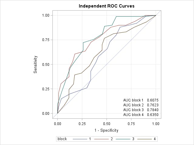
These statements combine the plot data from the two models and create a comparative plot which overlays the two ROC curves.

      data twoplots;
        set ROC12 ROC34;
        run;
      proc sgplot data=twoplots;
        series y=_sensit_ x=_1mspec_ / group=_roc_;
        run;

These statements combine the ROC information from the two models, then compute and display the test comparing the areas under the two ROC curves.

      data roctest2;
        set auc12;
        AUC1=area; s1=stderr;
        set auc34;
        AUC2=area; s2=stderr;
        Chisq=(auc1 - auc2)**2/(s1**2 + s2**2);
        Prob=1-probchi(Chisq,1); 
        format Prob pvalue6.; 
        Test="AUC1 - AUC2 = 0";
        output;
        stop;
        run;
      proc print noobs;
        var AUC1 AUC2 Test Chisq Prob;
        run;

The results of the test indicate that the two areas are not significantly different (p=0.7667).

Operating System and Release Information