Usage Note 39724: ROC analysis using validation data and cross validation
 |  |  |
The assessment of a model can be optimistically biased if the data used to fit the model are also used in the assessment of the model. Two ways of dealing with this are discussed and illustrated below. The first is to split the available data into training and validation data sets. The model is fit (trained) using the training data set and then assessed by using the model to score the validation data set. However, when the amount of data available is small, this can result in an unacceptably small training data set. Another option is cross validation which provides an unbiased assessment of the model without reducing the training data set.
The ROC (Receiver Operating Characteristic) curve and the area under the ROC curve (AUC) are commonly used to assess the performance of binary response models such as logistic models. This example illustrates the use of a validation data set and cross validation to produce an ROC curve and estimate its area.
See this note for an example that compares the areas under competing binary response models – a logistic generalized additive model that uses splines and an ordinary logistic model – that are fit to the same data.
For an extension of the AUC for multinomial models, see the MultAUC macro.
The DATA step below creates the data sets used in these examples. Data were gathered from four blocks. Data set TRAIN contains the data from the first three blocks and will be used as the training data set. Data set VALID contains the fourth block and will be used as the validation data set. Data set ALLDATA contains the complete set of data and will be used later to illustrate cross validation.
      data alldata train valid;
        input block entry lat lng n r @@;
        do i=1 to r;
          y=1;
          output alldata;
          if block<4 then output train;
          else output valid;
        end;
        do i=1 to n-r;
          y=0;
          output alldata;
          if block<4 then output train;
          else output valid;
        end;
        datalines;
        1 14 1 1  8 2    1 16 1 2  9 1
        1  7 1 3 13 9    1  6 1 4  9 9
        1 13 2 1  9 2    1 15 2 2 14 7
        1  8 2 3  8 6    1  5 2 4 11 8
        1 11 3 1 12 7    1 12 3 2 11 8
        1  2 3 3 10 8    1  3 3 4 12 5
        1 10 4 1  9 7    1  9 4 2 15 8
        1  4 4 3 19 6    1  1 4 4  8 7
        2 15 5 1 15 6    2  3 5 2 11 9
        2 10 5 3 12 5    2  2 5 4  9 9
        2 11 6 1 20 10   2  7 6 2 10 8
        2 14 6 3 12 4    2  6 6 4 10 7
        2  5 7 1  8 8    2 13 7 2  6 0
        2 12 7 3  9 2    2 16 7 4  9 0
        2  9 8 1 14 9    2  1 8 2 13 12
        2  8 8 3 12 3    2  4 8 4 14 7
        3  7 1 5  7 7    3 13 1 6  7 0
        3  8 1 7 13 3    3 14 1 8  9 0
        3  4 2 5 15 11   3 10 2 6  9 7
        3  3 2 7 15 11   3  9 2 8 13 5
        3  6 3 5 16 9    3  1 3 6  8 8
        3 15 3 7  7 0    3 12 3 8 12 8
        3 11 4 5  8 1    3 16 4 6 15 1
        3  5 4 7 12 7    3  2 4 8 16 12
        4  9 5 5 15 8    4  4 5 6 10 6
        4 12 5 7 13 5    4  1 5 8 15 9
        4 15 6 5 17 6    4  6 6 6  8 2
        4 14 6 7 12 5    4  7 6 8 15 8
        4 13 7 5 13 2    4  8 7 6 13 9
        4  3 7 7  9 9    4 10 7 8  6 6
        4  2 8 5 12 8    4 11 8 6  9 7
        4  5 8 7 11 10   4 16 8 8 15 7
      ;
ROC analysis using separate training and validation data sets
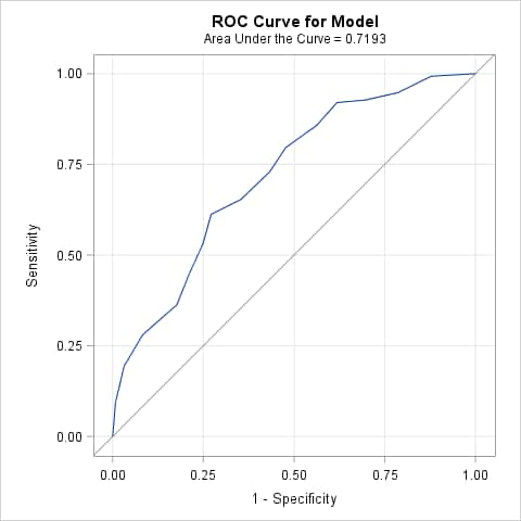
Begin by fitting the model to the training data set, TRAIN. Include a SCORE statement to apply the fitted model to the validation data set (VALID) and create a data set of predicted event probabilities (VALPRED). The OUTROC= options in the MODEL and SCORE statements produce plots of the ROC curves for the training and validation data sets (when ODS graphics is on) and also saves the ROC data in a data set. The point estimates of the areas under these two curves are given in the plots. If desired, adding the ROC statement produces a confidence interval for the area under the ROC curve for the training data. If the ROCCONTRAST statement is also added, then a test is provided of the hypothesis that the AUC of the model applied to the training data equals 0.5, which is the AUC of an uninformative model.
      ods graphics on;
      proc logistic data=train;
        model y(event="1") = entry / outroc=troc;
        score data=valid out=valpred outroc=vroc;
        roc; roccontrast;
        run;
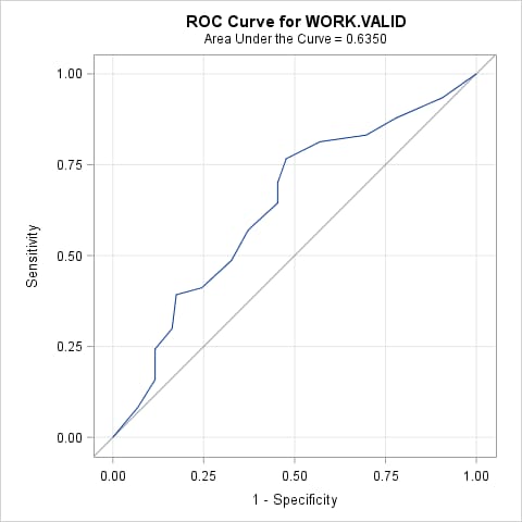
The AUC for the fitted model applied to the training data set is 0.7193. When applied to the validation data set, the AUC is 0.6350. The significant ROC contrast test (p<0.0001) indicates that the fitted model is better than the uninformative model when applied to the training data.
|
||||||||||||||||||||||||||||||||||||||||||||||||
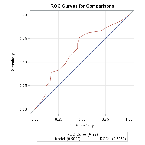
To obtain a confidence interval and test of the AUC for the validation data, a second PROC LOGISTIC step is needed. In this step, use the predicted event probabilities from scoring the validation data (in data set VALPRED) as the variable in the PRED= option in the ROC statement. Since Y=1 is specified as the event level in this example, the variable containing the predicted event probabilities is named P_1. By specifying no predictors in the MODEL statement, a model containing only an intercept is fitted. The area under this model is 0.5 which is the area of an uninformative model. Including the ROCCONTRAST statement compares the fitted and uninformative models applied to the validation data.
      proc logistic data=valpred;
        model y(event="1")=;
        roc pred=p_1;
        roccontrast;
        run;
The AUC from applying the fitted model to the validation data set is again shown to be 0.6350. The significant ROC contrast test (p=0.0009) indicates that the fitted model is better than the uninformative model when applied to the validation data.
|
||||||||||||||||||||||||||||||||||||||||||||||||
Beginning in SAS® 9.3, the point estimate of the AUC for the validation data can be obtained by specifying the FITSTAT option in the SCORE statement. The following statements produce AUC point estimates for both the training data set and the validation data set.
      proc logistic data=train;
        model y(event="1") = entry;
        score data=train fitstat;
        score data=valid fitstat;
        run;
If a test comparing the AUCs for the training and validation data is needed, this cannot be done using the ROCCONTRAST statement. The ROCCONTRAST statement employs a test needed when the ROC curves are correlated, such as when competing models are fit to the same data. The ROC curves from the model fit to the training data and applied to the validation data are not correlated curves, so a different test must be used. Comparison of uncorrelated curves is discussed and illustrated in this note.
|
||||||||||||||||||||||||||||||||||||||||||||||||
ROC analysis using cross validation
Assessment via cross validation is done by fitting the model to the complete data set and using the cross validated predicted probabilities to provide an ROC analysis. The cross validated predicted probability for an observation simulates the process of fitting the model ignoring that observation and then using the model fit to the remaining observations to compute the predicted probability for the ignored observation.
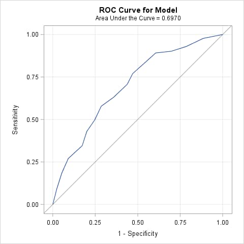
Beginning in SAS 9.4 TS1M3, you can specify the ROCOPTIONS(CROSSVALIDATE) option to produce an ROC curve and AUC estimate based on cross validated predicted probabilities. The following statements produce the ROC curve and AUC estimate using the complete data set (ALLDATA) without cross validation and then again with cross validation. Note that the cross validated area estimate is lower.
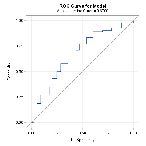
      proc logistic data=alldata plots(only)=roc;
        model y(event="1") = entry;
        run;

      proc logistic data=alldata rocoptions(crossvalidate) plots(only)=roc;
        model y(event="1") = entry;
        run;
  |
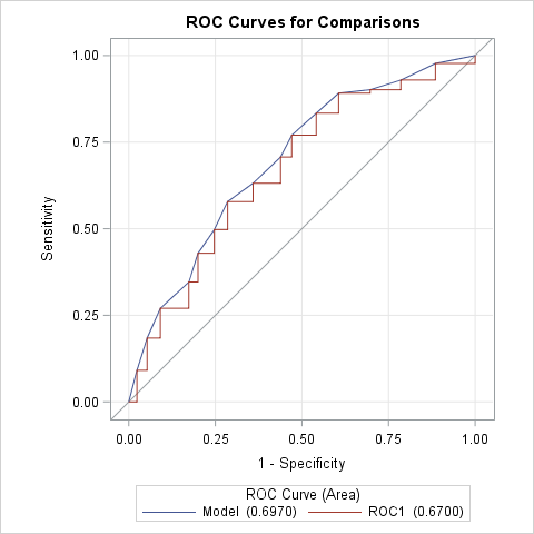
You can use the following approach in releases prior to SAS 9.4 TS1M3 or if you want to create an overlaid plot of the ROC curves and a comparison of the AUCs with and without cross validation. In the first LOGISTIC step below, the model is fit to the complete data (ALLDATA). The PREDPROBS=CROSSVALIDATE option in the OUTPUT statement creates a data set containing the cross validated predicted probabilities. The second LOGISTIC step refits the model (labeled Model) and produces its ROC curve and AUC estimate. Since Y=1 is specified as the event level in this example, the variable containing the cross validated predicted event probabilities is named XP_1. The PRED=XP_1 option in the ROC statement produces a second ROC curve (labeled ROC1) and AUC estimate based on the cross validated probabilities. The ROCCONTRAST statement tests the equality of the AUCs of the fitted model with and without cross validation.
      proc logistic data=alldata;
        model y(event="1") = entry;
        output out=preds predprobs=crossvalidate;
        run;
      proc logistic data=preds;
        model y(event="1") = entry;
        roc pred=xp_1;
        roccontrast;
        run;
Note that the AUC drops significantly (p<0.0001) from 0.697 to 0.670 when cross validation is used.
|
||||||||||||||||||||||||||||||||||||||||||||||||
Operating System and Release Information
| Product Family | Product | System | SAS Release | |
| Reported | Fixed* | |||
| SAS System | SAS/STAT | z/OS | ||
| OpenVMS VAX | ||||
| Microsoft® Windows® for 64-Bit Itanium-based Systems | ||||
| Microsoft Windows Server 2003 Datacenter 64-bit Edition | ||||
| Microsoft Windows Server 2003 Enterprise 64-bit Edition | ||||
| Microsoft Windows XP 64-bit Edition | ||||
| Microsoft® Windows® for x64 | ||||
| OS/2 | ||||
| Microsoft Windows 95/98 | ||||
| Microsoft Windows 2000 Advanced Server | ||||
| Microsoft Windows 2000 Datacenter Server | ||||
| Microsoft Windows 2000 Server | ||||
| Microsoft Windows 2000 Professional | ||||
| Microsoft Windows NT Workstation | ||||
| Microsoft Windows Server 2003 Datacenter Edition | ||||
| Microsoft Windows Server 2003 Enterprise Edition | ||||
| Microsoft Windows Server 2003 Standard Edition | ||||
| Microsoft Windows Server 2003 for x64 | ||||
| Microsoft Windows Server 2008 | ||||
| Microsoft Windows Server 2008 for x64 | ||||
| Microsoft Windows XP Professional | ||||
| Windows 7 Enterprise 32 bit | ||||
| Windows 7 Enterprise x64 | ||||
| Windows 7 Home Premium 32 bit | ||||
| Windows 7 Home Premium x64 | ||||
| Windows 7 Professional 32 bit | ||||
| Windows 7 Professional x64 | ||||
| Windows 7 Ultimate 32 bit | ||||
| Windows 7 Ultimate x64 | ||||
| Windows Millennium Edition (Me) | ||||
| Windows Vista | ||||
| Windows Vista for x64 | ||||
| 64-bit Enabled AIX | ||||
| 64-bit Enabled HP-UX | ||||
| 64-bit Enabled Solaris | ||||
| ABI+ for Intel Architecture | ||||
| AIX | ||||
| HP-UX | ||||
| HP-UX IPF | ||||
| IRIX | ||||
| Linux | ||||
| Linux for x64 | ||||
| Linux on Itanium | ||||
| OpenVMS Alpha | ||||
| OpenVMS on HP Integrity | ||||
| Solaris | ||||
| Solaris for x64 | ||||
| Tru64 UNIX | ||||
| Type: | Usage Note |
| Priority: | |
| Topic: | Analytics ==> Regression Analytics ==> Categorical Data Analysis SAS Reference ==> Procedures ==> LOGISTIC Analytics ==> Statistical Graphics |
| Date Modified: | 2020-03-11 16:02:31 |
| Date Created: | 2010-05-21 14:12:45 |