Usage Note 35189: Odds ratio, risk difference, and marginal effect for logistic model with polynomial or spline
 |  |  |
The following statements fit a logistic model which includes the linear and quadratic effects of X:
      proc logistic;
         model y = x x*x;
         run;
Note that you can also specify the quadratic model using bar notationNote:
model y = x|x;
The resulting model fit by PROC LOGISTIC can be written:
- LogOddsx = β0 + β1x + β2x2
For a continuous predictor, the odds ratio is typically computed as the change in odds for a unit increase in the predictor. Under the above model, a unit increase in X is
-
LogOddsx+1 = β0 + β1(x+1) + β2(x+1)2 = β0 + β1 + β1x + β2x2 + 2β2x + β2 = β0 + β1 + β1x + β2x2 + β2(2x+1)
Subtracting the model at X from the model at X+1 gives the linear combination of model parameters that estimates the difference in log odds for a unit increase in X. Also, note that the difference in log odds is the log odds ratio:
-
log(Oddsx+1/Oddsx) = LogOddsx+1 - LogOddsx = (β0 + β1 + β1x + β2x2 + β2(2x+1)) -
(β0 + β1x + β2x2)= β1 + β2(2x+1)
Exponentiating both sides shows that the odds ratio for a unit increase in X is:
- OddsRatiox+1 = Oddsx+1/Oddsx = exp(β1 + β2(2x+1))
Note that since the model is not linear, the change in odds for a unit change in X is not constant across X. Hence, the odds ratio is a function of X.
Because the CONTRAST statement can estimate and test linear combinations of model parameters, you can use the CONTRAST statement in PROC LOGISTIC to estimate the change in odds beginning at a given value of X. Adding the ESTIMATE=EXP option exponentiates the specified linear combination to produce the odds ratio estimate. You can also do this using the ESTIMATE statement. Add the EXP option to produce the odds ratio estimate and the CL option to provide confidence limits.
The CONTRAST and ESTIMATE statements below estimate the odds ratio (and a 95% confidence interval) for a unit change from X=3 to X=4. In both statements, the "1" following X is the multiplier of the X parameter (β1) in the above linear combination. The "7" following X*X is the multiplier of the X*X parameter (β2). For X=3, the multiplier of β2 is 2x+1=7.
      proc logistic;
         model y = x x*x;
         contrast 'Log OddsRatio for X' x 1 x*x 7 / estimate=exp;
         estimate 'Log OddsRatio for X' x 1 x*x 7 / exp cl;
         run;
You can do this more easily with the ODDSRATIO statement. Use the AT option to specify the starting value of the range over which the odds ratio should be computed. Include the UNITS statement to specify the amount of change over which the odds ratio should be computed. Without the UNITS statement, the odds ratio estimates the change in odds for a 1 unit increase in the variable. The following statements estimate the change in odds for a change in X from X=3 to X=4. The UNITS statement could be omitted in this case since a 1 unit change is requested. Also, you can use the EFFECT statement to produce a polynomial in X equivalent to the MODEL statement specification above. The following EFFECT statement creates an polynomial effect named QUAD that contains the linear and quadratic effects of X.
      proc logistic;
         effect quad=polynomial(x/degree=2);
         model y = quad;
         oddsratio x / at(x=3);
         units x=1;
         run;
Example
The following data are presented and analyzed using a generalized additive model in the PROC GAM documentation. The data used in this example are based on a study by Bell et al. (1994). Bell and his associates studied the result of multiple-level thoracic and lumbar laminectomy, a corrective spinal surgery commonly performed on children. The data in the study consist of retrospective measurements on 83 patients. The specific outcome of interest is the presence (1) or absence (0) of kyphosis, defined as a forward flexion of the spine of at least 40 degrees from vertical. In this example, the beginning of the range of vertebrae levels involved in the operation (StartVert) is used as a predictor of kyphosis. The following statements create the kyphosis data set.
      data kyphosis;
         input Age StartVert NumVert Kyphosis @@;
         datalines;
         71  5  3  0     158 14 3 0    128 5   4 1
         2   1  5  0     1   15 4 0    1   16  2 0
         61  17 2  0     37  16 3 0    113 16  2 0
         59  12 6  1     82  14 5 1    148 16  3 0
         18  2  5  0     1   12 4 0    243 8   8 0
         168 18 3  0     1   16 3 0    78  15  6 0
         175 13 5  0     80  16 5 0    27  9   4 0
         22  16 2  0     105 5  6 1    96  12  3 1
         131 3  2  0     15  2  7 1    9   13  5 0
         12  2 14  1     8   6  3 0    100 14  3 0
         4   16 3  0     151 16 2 0    31  16  3 0
         125 11 2  0     130 13 5 0    112 16  3 0
         140 11 5  0     93  16 3 0    1   9   3 0
         52  6  5  1     20  9  6 0    91  12  5 1
         73  1  5  1     35  13 3 0    143 3   9 0
         61  1  4  0     97  16 3 0    139 10  3 1
         136 15 4  0     131 13 5 0    121 3   3 1
         177 14 2  0     68  10 5 0    9   17  2 0
         139 6  10 1     2   17 2 0    140 15  4 0
         72  15 5  0     2   13 3 0    120 8   5 1
         51  9  7  0     102 13 3 0    130 1   4 1
         114 8  7  1     81  1  4 0    118 16  3 0
         118 16 4  0     17  10 4 0    195 17  2 0
         159 13 4  0     18  11 4 0    15  16  5 0
         158 15 4  0     127 12 4 0    87  16  4 0
         206 10 4  0     11  15 3 0    178 15  4 0
         157 13 3  1     26  13 7 0    120 13  2 0
         42  6  7  1     36  13 4 0
         ;
Odds Ratio for Increase in Predictor
The following statements fit a logistic model involving linear and quadratic effects of StartVert. The ODDSRATIO and UNITS statements request odds ratio estimates for increases of one and two units in StartVert at each of two points, 5 and 10. Included are four sets of CONTRAST statements which estimate the same odds ratios as the ODDSRATIO statement. In each set, two CONTRAST statements estimate the log odds of kyphosis at two StartVert values, and the third CONTRAST statement estimates the odds ratio using coefficients that are the difference of the previous two CONTRASTs. The OUTPUT statement saves the predicted logits (log odds) from the fitted model, and the plot produced by PROC SGPLOT shows the estimated effect of StartVert on the logit scale. The EFFECT statement is not used here to produce the polynomial in StartVert since effects specified in the CONTRAST and ESTIMATE statements must appear in the MODEL statement.
      proc logistic data=kyphosis;
         model Kyphosis(event="1") = StartVert|StartVert;
         oddsratio StartVert / at(StartVert=5 10);
         units StartVert=1 2;

         /* Odds ratio for change in StartVert from 10 to 11 */
         contrast 'logOdds@x=10' intercept 1 startvert 10 startvert*startvert 100 / estimate=both;
         contrast 'logOdds@x=11' intercept 1 startvert 11 startvert*startvert 121 / estimate=both;
         contrast 'logOdds@11-logOdds10' startvert 1 startvert*startvert 21 / estimate=both;

         /* Odds ratio for change in StartVert from 5 to 6 */
         contrast 'logOdds@x=5' intercept 1 startvert 5 startvert*startvert 25 / estimate=both;
         contrast 'logOdds@x=6' intercept 1 startvert 6 startvert*startvert 36 / estimate=both;
         contrast 'logOdds@6-logOdds@5' startvert 1 startvert*startvert 11 / estimate=both;

         /* Odds ratio for change in StartVert from 10 to 12 */
         contrast 'logOdds@x=10' intercept 1 startvert 10 startvert*startvert 100 / estimate=both;
         contrast 'logOdds@x=12' intercept 1 startvert 12 startvert*startvert 144 / estimate=both;
         contrast 'logOdds@12-logOdds10' startvert 2 startvert*startvert 44 / estimate=both;

         /* Odds ratio for change in StartVert from 5 to 7 */
         contrast 'logOdds@x=5' intercept 1 startvert 5 startvert*startvert 25 / estimate=both;
         contrast 'logOdds@x=7' intercept 1 startvert 7 startvert*startvert 49 / estimate=both;
         contrast 'logOdds@7-logOdds@5' startvert 2 startvert*startvert 24 / estimate=both;
         output out=logits xbeta=logit;
         effectplot / link;
         effectplot;
         run;
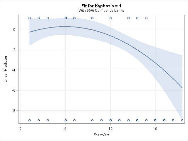
The Analysis of Maximum Likelihood Estimates table shows that the quadratic effect of StartVert is significant (p=0.0357). The plot produced by the first EFFECTPLOT statement shows the fitted quadratic curve on the log odds (linear predictor) scale. The LINK option requests that the vertical axis use the link function (logit or log odds in this case) scale.
 |
||||||||||||||||||||||||||||||
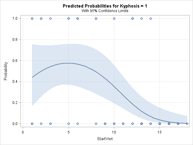
The second EFFECTPLOT statement shows the fitted curve on the mean (probability) scale.
 |
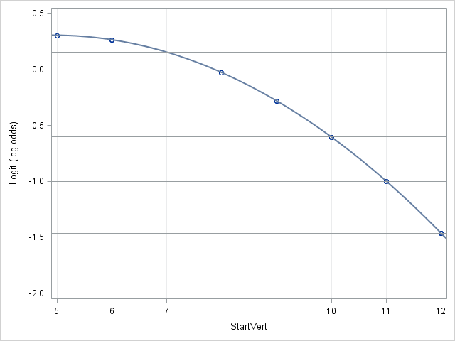
The following statements reproduce the plot from the first EFFECTPLOT statement and focuses in on the 5 to 12 range of StartVert.
      proc sort data=logits;
         by StartVert;
         run;

      proc sgplot data=logits;
         pbspline y=logit x=StartVert / nolegfit;
         refline -.603 -.998 .305 .266 -1.464 .155 / axis=y;
         refline 5 6 7 10 11 12/ axis=x transparency=.8;
         yaxis label="Logit (log odds)" values=(-2 to .5 by .5);
         xaxis values=(5 6 7 10 11 12);
         run;
The plot of the fitted model on the log odds scale includes reference lines showing the log odds at StartVert values in two regions of interest — 5, 6, and 7 where the fitted curve is just starting to fall, and at 10, 11, and 12 where the curve is falling more sharply.
 |
The ODDSRATIO statement produces the following table. The odds ratios for one and two unit increases in StartVert are estimated at two different points, 5 and 10.
|
||||||||||||||||||||||||
In the table of results from the CONTRAST statements below, the first row gives the estimate of the log odds (-0.6034) at a StartVert ("x" in the label at left) value of 10. You can see this value in the plot above from the line intersecting the curve at StartVert=10. Exponentiating this log odds gives the estimate in the second row (Type=EXP) of the odds (0.5469) at this point. Similarly, at StartVert=11 the log odds estimate is -0.9981 and the odds estimate is 0.3686. The fifth and sixth rows contain estimates of the difference in log odds at StartVert=10 and 11 (-.9981-(-.6034) = -0.3947) and the resulting odds ratio estimate (0.3686/0.5469 = 0.6739) from exponentiating that difference. The next set of rows of the table do the same for a unit increase in StartVert from 5 to 6. Note in the plot that the log odds of kyphosis changes relatively little from 5 to 6, but changes much more substantially from 10 to 11. The small change at 5 is confirmed by the odds ratio estimate being close to 1 (0.9610), with a large p-value (p=0.6930), and a confidence interval that includes 1 (0.7886, 1.1710). At StartVert=10, the odds ratio estimate is not close to 1 (0.6739; p=0.0007), and has a confidence interval that doesn't include 1 (0.5360, 0.8473).
The next two sets of rows in the table estimate the odds ratios for changes of two units from 5 and 10 respectively. Similar results are obtained showing a more extreme (0.860) but still nonsignificant change in odds from 5 to 7. The change in odds from 10 to 12 is also more extreme (0.423) and highly significant.
Notice that all odds ratio estimates and confidence intervals from the CONTRAST statements match the results produced by the ODDSRATIO statement.
|
||||||||||||||||||||||||||||||||||||||||||||||||||||||||||||||||||||||||||||||||||||||||||||||||||||||||||||||||||||||||||||||||||||||||||||||||||||||||||||||||||||||||||||||||||||||||||||||||||||||||||||||||||||||||||||||||||||||||||||||||||||||||||||||||||||
The same results (except for the individual log odds estimates) are produced by these statements:
      proc logistic data=kyphosis;
          effect quad=polynomial(StartVert/degree=2);
          model Kyphosis(event="1") = quad;
          oddsratio StartVert / at(StartVert=5 10);
          units StartVert=1 2;
          run;
Marginal Effect of Predictor
When looking at the plot of the model on the probability of kyphosis, Predicted Probabilities for Kyphosis=1 shown above, perhaps of more intuitive interest than the odds ratio is the instantaneous change in the probability of kyphosis at a specific value of StartVert. It is the slope of the line tangent to the curve of the fitted model at specific values such as 5 or 10. This is the marginal effect of StartVert at those values and can be obtained using the Margins macro.
The following statements refit the quadratic logistic model and estimate and test the marginal effect of StartVert at values 5 and 10. The same analysis can be done without the initial DATA step by specifying atwhere=(StartVert in (5,10)) instead of atdata=at, but this requires that values 5 and 10 appear at least once in the StartVert variable in the input data set.
     data at;
        do startvert=5,10;
           output;
        end;
        run;
     %Margins(data     = kyphosis,
              response = kyphosis,
              roptions = event='1',
              dist     = binomial,
              model    = StartVert|StartVert,
              effect   = StartVert, at=StartVert, atdata=at,
              options  = cl nomodel noprintbyat)
Compare the following estimated marginal effects to the plot of the model on the probability of kyphosis above. The slope of a line drawn tangent to the probability curve at StartVert=5 is obviously nearly flat and this is confirmed by the estimated marginal effect (-0.0011) at that point. The test that it differs from zero is far from significant (p=0.9697). However, at StartVert=10, the probability curve is dropping noticeably. The estimated marginal effect at that point is -0.0821 and is now significantly different from zero (p=0.0032).
|
Risk Difference for Unit Increase in Predictor
A rough approximation of the marginal effect is the risk difference (difference in event probabilities) over a unit change in StartVert centered at each of the two points. This can be done by specifying a two-row L matrix in the ESTIMATE for each point. The first row estimates the log odds 0.5 units below the point and the second estimates the log odds 0.5 units above the point. The NLMeans macro can then compute the risk difference. It requires the coefficients provided by the E option in each ESTIMATE statement and saved by the ODS OUTPUT statement. The saved model, provided by the STORE statement, is also required.
     proc logistic data=kyphosis;
        model Kyphosis(event="1") = StartVert|StartVert;
        estimate  '4.5' intercept 1 startvert 4.5 startvert*startvert 20.25,
                  '5.5' intercept 1 startvert 5.5 startvert*startvert 30.25 / e;
        estimate  '9.5' intercept 1 startvert 9.5 startvert*startvert 90.25,
                  '10.5' intercept 1 startvert 10.5 startvert*startvert 110.25 / e;
        ods output coef=c;
        store log;
        run;
     %NLMeans(instore=log, coef=c, link=logit, options=reverse)
The results from the NLMeans macro are very similar to the marginal effects from the Margins macro above.
|
Odds Ratio for Increase in Predictor in a Spline Model
A similar analysis could be done using a less restrictive spline effect for StartVert rather than a polynomial effect.
      proc logistic data=kyphosis;
          effect s=spline(StartVert/naturalcubic);
          model Kyphosis(event="1") = s;
          oddsratio StartVert / at(StartVert=5 10);
          units StartVert=1 2;
          effectplot / link;
          effectplot;
          run;
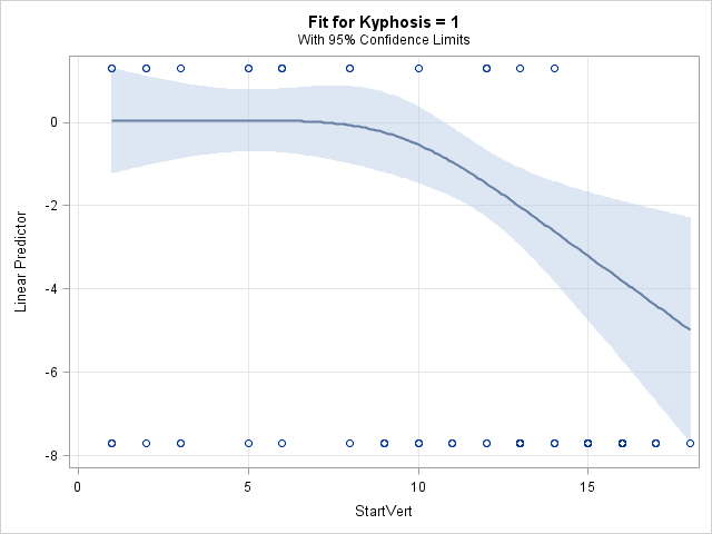
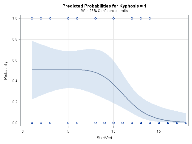
This model using the spline effect of StartVert produces similar odds ratio estimates and similar fitted curves, though the curves can be somewhat flatter at lower values of StartVert since the spline is not restricted to a polynomial shape.
  |
||||||||||||||||||||||||
_____
Note: Higher-order models can be compactly written in similar fashion. For example, a fourth-order model can be specified as:
-
model y = x|x|x|x;
Operating System and Release Information
| Product Family | Product | System | SAS Release | |
| Reported | Fixed* | |||
| SAS System | SAS/STAT | Microsoft Windows 95/98 | ||
| Microsoft Windows 2000 Advanced Server | ||||
| OS/2 | ||||
| Microsoft® Windows® for x64 | ||||
| Microsoft Windows Server 2003 Enterprise 64-bit Edition | ||||
| Microsoft Windows XP 64-bit Edition | ||||
| z/OS | ||||
| OpenVMS VAX | ||||
| Microsoft Windows Server 2003 Datacenter 64-bit Edition | ||||
| Microsoft® Windows® for 64-Bit Itanium-based Systems | ||||
| Microsoft Windows 2000 Datacenter Server | ||||
| Microsoft Windows 2000 Server | ||||
| Microsoft Windows 2000 Professional | ||||
| Microsoft Windows NT Workstation | ||||
| Microsoft Windows Server 2003 Datacenter Edition | ||||
| Microsoft Windows Server 2003 Enterprise Edition | ||||
| Microsoft Windows Server 2003 Standard Edition | ||||
| Microsoft Windows XP Professional | ||||
| Windows Millennium Edition (Me) | ||||
| Windows Vista | ||||
| 64-bit Enabled AIX | ||||
| 64-bit Enabled HP-UX | ||||
| 64-bit Enabled Solaris | ||||
| ABI+ for Intel Architecture | ||||
| AIX | ||||
| HP-UX | ||||
| HP-UX IPF | ||||
| IRIX | ||||
| Linux | ||||
| Linux for x64 | ||||
| Linux on Itanium | ||||
| OpenVMS Alpha | ||||
| OpenVMS on HP Integrity | ||||
| Solaris | ||||
| Solaris for x64 | ||||
| Tru64 UNIX | ||||
| Type: | Usage Note |
| Priority: | |
| Topic: | SAS Reference ==> Procedures ==> LOGISTIC Analytics ==> Categorical Data Analysis Analytics ==> Regression |
| Date Modified: | 2022-06-14 09:05:29 |
| Date Created: | 2009-03-18 15:32:29 |