These examples appear in Chapter 8 of The Little SAS Book: A Primer, Fourth Edition.

Before you run the examples, open the zip file under the Downloads tab. Using the list below, create the folders and copy the data files so that the data are available during your SAS session.

Create the folder c:\MyRawData and copy these files to it:

             
   Address.dat          IceCreamSales.dat         Shakespeare.dat      
   Admit.dat            IceCreamSales2.dat        Shoe.dat             
   AllScores.dat        Lengths.dat               Shoesales.dat        
   Artists.dat          Library.dat               South.dat             
   Baseball.dat         LibraryBooks.dat          Speed.dat              
   Basketball.dat       Mag.dat                   Survey.dat             
   Boats2.dat           Mens5000.dat              Temperature.dat      
   Boats.dat            Mountains.dat             Temps.dat             
   Books.dat            Movies.dat                ToadJump.dat         
   Bus.dat              NatPark.Dat               Tomatoes.dat          
   Candy.dat            NewAdmit.dat              Traffic.dat          
   Cars.dat             North.dat                 Train.dat             
   Choc.dat             Olympic1500.dat           Transpos.dat         
   Chocolate.dat        OnionRing.dat             TropicalSales.dat        
   Chocsales.dat        Onions.dat                UsedCars.dat         
   Coffee.dat           OrdersQ3.dat              Walk.dat             
   Criterium.dat        Parks.dat                 WBRK.dat             
   CustAddress.dat      Picbooks.dat              Zoo.dat                
   Disc.dat             Precipitation.dat                                  
   Exercise.dat         President.dat             Bands.csv             
   Flowers.dat          Pumpkin.dat               Bands2.csv             
   Games.dat            Records.dat               Women.csv            
   Garden.dat           Scores.dat                                     
   Home.dat             SeaLife.dat                                     
                                                                       
 

Create the folder c:\MyFiles and copy this file to it: Baseball.xls

Create the folder c:\MyWebLogs and copy this file to it: dogweblogs.txt

Create the folder c:\MyExcelFiles and copy these files to it: Baseball.xls, OnionRing.xls

Create the folder c:\MyData to store files when you run examples

Create the folder c:\MyHTML to store files when you run examples

Create the folder c:\MyHTMLFiles to store files when you run examples

Create the folder c:\MyPDFFiles to store files when you run examples

Create the folder c:\MyRTFFiles to store files when you run examples

Create the folder c:\MySASLib and copy this file to it: TropicalSales.dat

---

Section 8.2

DATA chocolate;
   INFILE 'c:\MyRawData\Choc.dat';
   INPUT AgeGroup $ FavoriteFlavor $ Uniqueness @@;
RUN;

* Bar charts for favorite flavor;
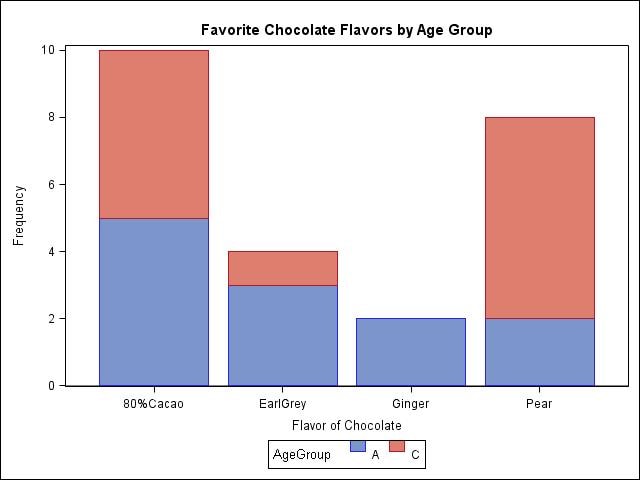
PROC SGPLOT DATA = chocolate;
   VBAR FavoriteFlavor / GROUP = AgeGroup;
   LABEL FavoriteFlavor = 'Flavor of Chocolate';
   TITLE 'Favorite Chocolate Flavors by Age Group';
RUN;
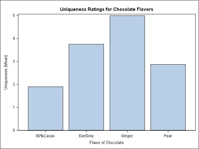
PROC SGPLOT DATA = chocolate;
   VBAR FavoriteFlavor / RESPONSE = Uniqueness STAT = MEAN;
   LABEL FavoriteFlavor = 'Flavor of Chocolate';
   TITLE 'Uniqueness Ratings for Chocolate Flavors';
RUN;

---

Section 8.3

DATA bikerace;
   INFILE 'c:\MyRawData\Criterium.dat';
   INPUT Division $ NumberLaps @@;
RUN;
* Create histogram;
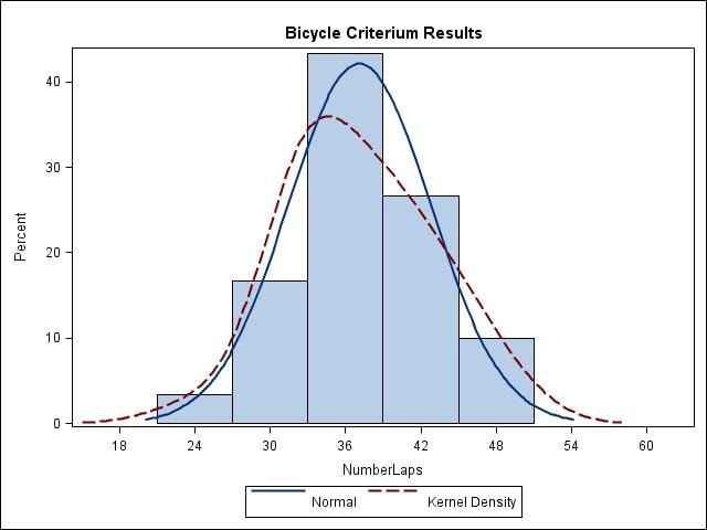
PROC SGPLOT DATA = bikerace;
   HISTOGRAM NumberLaps / SHOWBINS;
   DENSITY NumberLaps;
   DENSITY NumberLaps / TYPE = KERNEL;
   TITLE 'Bicycle Criterium Results';
RUN;
* Create box plot;
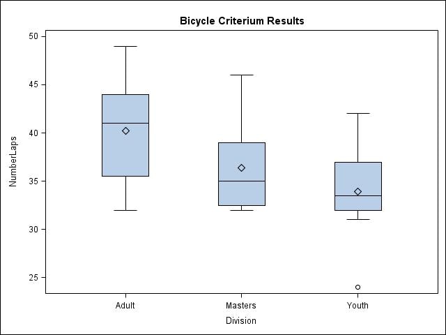
PROC SGPLOT DATA = bikerace;
   VBOX NumberLaps / CATEGORY = Division;
   TITLE 'Bicycle Criterium Results';
RUN;

---

Section 8.4

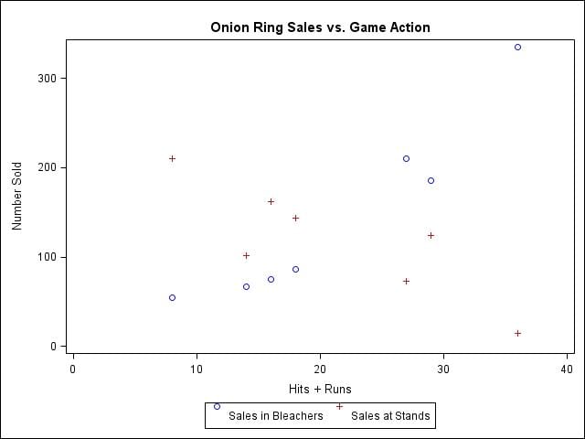
DATA onionrings;
   INFILE 'c:\MyRawData\Onions.dat';
   INPUT VisTeam $ 1-20 CSales BSales OurHits VisHits OurRuns VisRuns;
   Action = OurHits + VisHits + OurRuns + VisRuns;
RUN;

* Plot Bleacher Sales by Action;
PROC SGPLOT DATA = onionrings;
   SCATTER X = Action Y = BSales;
   SCATTER X = Action Y = CSales;
   XAXIS LABEL = 'Hits + Runs' VALUES = (0 TO 40 BY 10);
   YAXIS LABEL = 'Number Sold';
   LABEL BSales = 'Sales in Bleachers'
         CSales = 'Sales at Stands';
   TITLE 'Onion Ring Sales vs. Game Action';
RUN;

---

Section 8.5

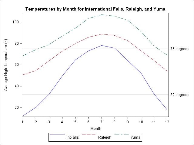
DATA temperatures;
   INFILE 'c:\MyRawData\Temps.dat';
   INPUT Month IntFalls Raleigh Yuma @@;
RUN;

* Plot average high and low temperatures by city;
PROC SGPLOT DATA = temperatures;
   SERIES X = Month Y = IntFalls;
   SERIES X = Month Y = Raleigh;
   SERIES X = Month Y = Yuma;
   REFLINE 32 75 / TRANSPARENCY = 0.5 LABEL = ('32 degrees' '75 degrees');
   XAXIS TYPE = DISCRETE;
   YAXIS LABEL = 'Average High Temperature (F)';
   TITLE 'Temperatures by Month for International Falls, '
      'Raleigh, and Yuma';
RUN;

---

Section 8.6

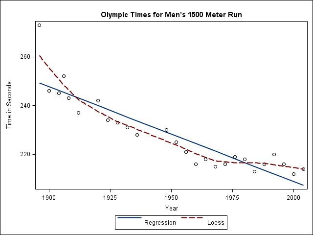
DATA Olympic1500;
  INFILE 'C:\MyRawData\Olympic1500.dat';
  INPUT Year Men @@;
RUN;
PROC SGPLOT DATA=Olympic1500;
  REG X=Year Y=Men;
  LOESS X=Year Y=Men / NOMARKERS;
  YAXIS LABEL='Time in Seconds';
  TITLE "Olympic Times for Men's 1500 Meter Run";
RUN;
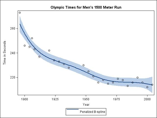
PROC SGPLOT DATA=Olympic1500;
  PBSPLINE X=Year Y=Men/CLM NOLEGCLM;
  YAXIS LABEL='Time in Seconds';
  TITLE "Olympic Times for Men's 1500 Meter Run";
RUN;

---

Section 8.7

DATA class;
   INFILE 'c:\MyRawData\Scores.dat';
   INPUT Score @@;
RUN;
PROC UNIVARIATE DATA = class;
   VAR Score;
   TITLE;
RUN;

---

Section 8.8

ODS GRAPHICS ON;
PROC UNIVARIATE DATA = class;
   VAR Score;
   HISTOGRAM Score/NORMAL;
   PROBPLOT Score;
   TITLE;
RUN;

---

Section 8.9

DATA booklengths;   
   INFILE 'c:\MyRawData\Picbooks.dat';
   INPUT NumberOfPages @@;
RUN;
*Produce summary statistics;
PROC MEANS DATA=booklengths N MEAN MEDIAN CLM ALPHA=.10;
   TITLE 'Summary of Picture Book Lengths';
RUN;

---

Section 8.10

DATA bus;
   INFILE 'c:\MyRawData\Bus.dat';
   INPUT BusType $  OnTimeOrLate $ @@;
RUN;
PROC FREQ DATA = bus;
   TABLES BusType * OnTimeOrLate / CHISQ;
   TITLE;
RUN;

---

Section 8.11

ODS GRAPHICS ON;
PROC FREQ DATA = bus;
   TABLES BusType * OnTimeOrLate;
   TABLES BusType * OnTimeOrLate / PLOTS=FREQPLOT(TWOWAY=GROUPHORIZONTAL);
   TITLE;
RUN;

---

Section 8.12

DATA class;
   INFILE 'c:\MyRawData\Exercise.dat';
   INPUT Score Television Exercise @@;
RUN;
PROC CORR DATA = class;
   VAR Television Exercise;
   WITH Score;
   TITLE 'Correlations for Test Scores';
   TITLE2 'With Hours of Television and Exercise';
RUN;

---

Section 8.13

ODS GRAPHICS ON;
PROC CORR DATA = class PLOTS = (SCATTER MATRIX);
   VAR Television Exercise;
   WITH Score;
   TITLE 'Correlations for Test Scores';
   TITLE2 'With Hours of Television and Exercise';
RUN;
 

---

Section 8.14

DATA hits;
   INFILE 'c:\MyRawData\Baseball.dat';
   INPUT Height Distance @@;
RUN;
* Perform regression analysis;
PROC REG DATA = hits;
   MODEL Distance = Height;
   TITLE 'Results of Regression Analysis';
RUN;

---

Section 8.15

ODS GRAPHICS ON;
PROC REG DATA = hits PLOTS(ONLY) = (DIAGNOSTICS FITPLOT);
   MODEL Distance = Height;
   TITLE 'Results of Regression Analysis';
RUN;

---

Section 8.16

DATA basket;
   INFILE 'c:\MyRawData\Basketball.dat';
   INPUT Team $ Height @@;
RUN;
* Use ANOVA to run one-way analysis of variance;
ODS GRAPHICS ON;
PROC ANOVA DATA = basket;
   CLASS Team;
   MODEL Height = Team;
   MEANS Team / SCHEFFE;
   TITLE "Girls' Heights on Basketball Teams";
RUN;

---

Section 8.17

PROC ANOVA DATA = basket;
   CLASS Team;
   MODEL Height = Team;
   MEANS Team / SCHEFFE;
   TITLE "Girls’ Heights on Basketball Teams";
RUN;

---

The sample is authored by Lora D. Delwiche and Susan J. Slaughter.
Their book The Little SAS Book: A Primer, Fourth Edition is available for sale in our online bookstore.

---

These sample files and code examples are provided by SAS Institute Inc. "as is" without warranty of any kind, either express or implied, including but not limited to the implied warranties of merchantability and fitness for a particular purpose. Recipients acknowledge and agree that SAS Institute shall not be liable for any damages whatsoever arising out of their use of this material. In addition, SAS Institute will provide no support for the materials contained herein.

---

---

These sample files and code examples are provided by SAS Institute Inc. "as is" without warranty of any kind, either express or implied, including but not limited to the implied warranties of merchantability and fitness for a particular purpose. Recipients acknowledge and agree that SAS Institute shall not be liable for any damages whatsoever arising out of their use of this material. In addition, SAS Institute will provide no support for the materials contained herein.

Section 8.2, Output







Section 8.3, Output






Section 8.4, Output




Section 8.5, Output




Section 8.6, Output





Section 8.7, Output
                                    The UNIVARIATE Procedure
                                        Variable:  Score

                                             Moments

                 N                          30    Sum Weights                 30
                 Mean               74.6333333    Sum Observations          2239
                 Std Deviation      12.5848385    Variance            158.378161
                 Skewness           -0.3495061    Kurtosis            0.10385765
                 Uncorrected SS         171697    Corrected SS        4592.96667
                 Coeff Variation    16.8622222    Std Error Mean      2.29766665

                                   Basic Statistical Measures

                         Location                    Variability
                     Mean     74.63333     Std Deviation           12.58484
                     Median   74.50000     Variance               158.37816
                     Mode     73.00000     Range                   56.00000
                                           Interquartile Range     17.00000

                                   Tests for Location: Mu0=0

                        Test           -Statistic-    -----p Value------
                        Student's t    t  32.48223    Pr > |t|    <.0001
                        Sign           M        15    Pr >= |M|   <.0001
                        Signed Rank    S     232.5    Pr >= |S|   <.0001

                                    Quantiles (Definition 5)

                                     Quantile      Estimate
                                     100% Max         100.0
                                     99%              100.0
                                     95%               92.0
                                     90%               90.0
                                     75% Q3            84.0
                                     50% Median        74.5
                                     25% Q1            67.0
                                     10%               56.0
                                     5%                54.0
                                     1%                44.0
                                     0% Min            44.0
                                
                                      Extreme Observations

                              ----Lowest----        ----Highest---

                              Value      Obs        Value      Obs

                                 44        6           87       21
                                 54       24           90        5
                                 56       20           90       13
                                 56        1           92        9
                                 64       28          100       23


Section 8.8, Output






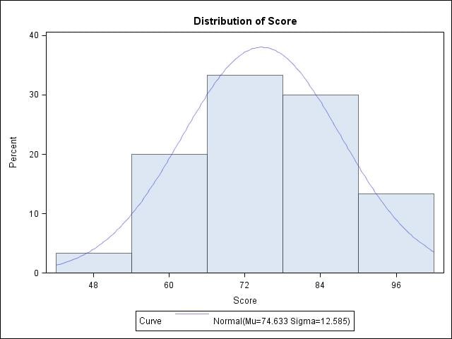
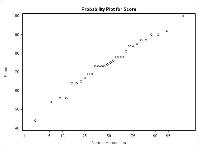
Section 8.9, Output  



Section 8.10, Output


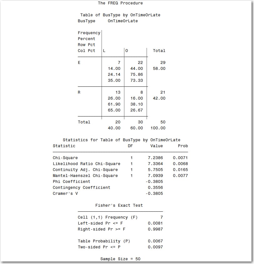
Section 8.11, Output





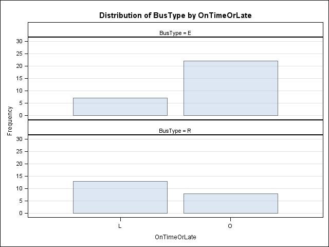
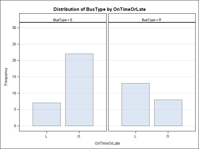
Section 8.12, Output
                                      
                                  Correlations for Test Scores
                              With Hours of Television and Exercise

                                       The CORR Procedure

                            1 With Variables:    Score
                            2      Variables:    Television Exercise

                                       Simple Statistics

  Variable             N          Mean       Std Dev           Sum       Minimum       Maximum

  Score               30      74.63333      12.58484          2239      44.00000     100.00000
  Television          30       5.10000       2.33932     153.00000             0       9.00000
  Exercise            30       2.83333       1.94906      85.00000             0       7.00000

                            Pearson Correlation Coefficients, N = 30
                                   Prob > |r| under H0: Rho=0

                                          Television      Exercise

                               Score        -0.55390       0.79733
                                             0.0015        0.0001
Section 8.13, Output





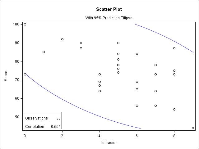
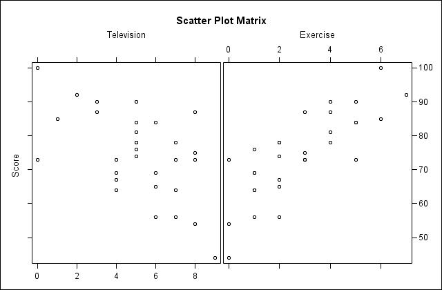
Section 8.14, Output
 
                                 Results of Regression Analysis

                                        The REG Procedure
                                          Model: MODEL1
                                  Dependent Variable: Distance

                                      Analysis of Variance

                                             Sum of           Mean
         Source                   DF        Squares         Square    F Value    Pr > F

         Model                     1     1365.50831     1365.50831      16.86    0.0003
         Error                    28     2268.35836       81.01280
         Corrected Total          29     3633.86667

                      Root MSE              9.00071    R-Square     0.3758
                      Dependent Mean      130.73333    Adj R-Sq     0.3535
                      Coeff Var             6.88479

                                      Parameter Estimates

                                   Parameter       Standard
              Variable     DF       Estimate          Error    t Value    Pr > |t|

              Intercept     1      -11.00859       34.56363      -0.32      0.7525
              Height        1        2.89466        0.70506       4.11      0.0003


Section 8.15, Output





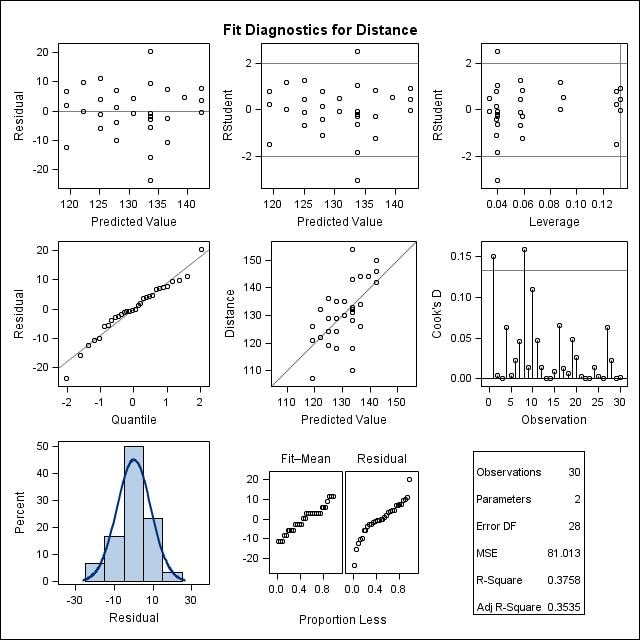
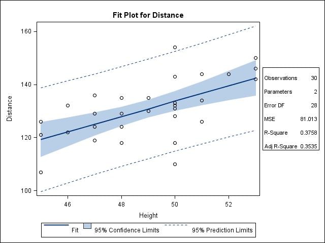
Section 8.16, Output





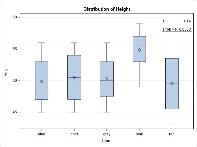
Section 8.17, Output




                                  
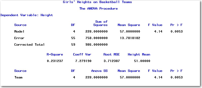
                               Girls' Heights on Basketball Teams

                                      The ANOVA Procedure

                                    Scheffe's Test for Height

                 NOTE: This test controls the Type I experimentwise error rate.

                             Alpha                              0.05
                             Error Degrees of Freedom             55
                             Error Mean Square              13.78182
                             Critical Value of F             2.53969
                             Minimum Significant Difference   4.8306

                   Means with the same letter are not significantly different.

                     Scheffe Grouping          Mean      N    Team

                                    A        54.833     12    pink
                                    A
                               B    A        50.500     12    gold
                               B    A
                               B    A        50.333     12    gray
                               B
                               B             49.833     12    blue
                               B
                               B             49.500     12    red
                              

Download the zip file in order to run these samples - zip file.

This sample shows you how to produce high-quality graphics with very little effort. General topics include creating appropriate graphics for your analyses and creating stand-alone graphs that are not included in the output of a statistical procedure.

Type:

Sample

Date Modified:	2009-01-29 17:20:07
Date Created:	2009-01-27 14:15:29

Operating System and Release Information

Product Family	Product	Host	SAS Release
			Starting	Ending
SAS System	Base SAS	z/OS
		OpenVMS VAX
		Microsoft® Windows® for 64-Bit Itanium-based Systems
		Microsoft Windows Server 2003 Datacenter 64-bit Edition
		Microsoft Windows Server 2003 Enterprise 64-bit Edition
		Microsoft Windows XP 64-bit Edition
		Microsoft® Windows® for x64
		OS/2
		Microsoft Windows 95/98
		Microsoft Windows 2000 Advanced Server
		Microsoft Windows 2000 Datacenter Server
		Microsoft Windows 2000 Server
		Microsoft Windows 2000 Professional
		Microsoft Windows NT Workstation
		Microsoft Windows Server 2003 Datacenter Edition
		Microsoft Windows Server 2003 Enterprise Edition
		Microsoft Windows Server 2003 Standard Edition
		Microsoft Windows XP Professional
		Windows Millennium Edition (Me)
		Windows Vista
		64-bit Enabled AIX
		64-bit Enabled HP-UX
		64-bit Enabled Solaris
		ABI+ for Intel Architecture
		AIX
		HP-UX
		HP-UX IPF
		IRIX
		Linux
		Linux for x64
		Linux on Itanium
		OpenVMS Alpha
		OpenVMS on HP Integrity
		Solaris
		Solaris for x64
		Tru64 UNIX