Sample 25017: Nonparametric comparison of areas under correlated ROC curves
 |  |  |  |  |
Nonparametric comparison of areas under correlated ROC curves
| Contents: | Purpose / History / Requirements / Usage / Details / Limitations / Missing Values / See Also / References |
NOTE: Beginning in SAS 9.2, comparison of areas under correlated ROC curves can be done using the ROC and ROCCONTRAST statements in PROC LOGISTIC. Examples are provided in the Results tab. See the PROC LOGISTIC documentation for additional details and examples.
NOTE: Indicated portions of the SAS/IML code in this sample program were provided, and are supported, by the author D.M. DeLong (see REFERENCES below).
- PURPOSE:
- Nonparametric comparison of areas under correlated ROC curves. Provides point and confidence interval estimates of each curve's area and of the pairwise differences among the areas. Tests of the pairwise differences are also given. Any contrast among the areas may be estimated and tested.
- HISTORY:
-
Version Update Notes 1.7 Fixed row labeling when CONTRAST= option is specified. 1.6 Removed computation of estimated correlations to avoid problems with use of intercept-only model. Fix to automatic check for new version. 1.5 Fixed subscript error in RNAME with 15 or more data sets and XBETA variables. Added automatic check for new version. 1.4 Corrected errors with default contrast and only one variable specified in VAR=. The single area is now estimated and tested. 1.3 Added confidence intervals for each area. Added ALPHA= parameter to control confidence level. Default contrasts are now all pairwise differences. Added table of confidence intervals and tests of each contrast row. 1.2 Put original author's code in macro form. Allow input of several data sets to compare several models which may each have multiple predictors. Default contrast set generated. Added DETAILS= parameter to minimize default output. Creates macro variable with overall p-value. - REQUIREMENTS:
- Version 7 or later of Base SAS and SAS/IML.
- USAGE:
-
Follow the instructions in the Downloads tab of this
sample to save the %ROC macro definition. Replace the text within quotes in the following statement with the location of the %ROC macro definition file on your system. In your SAS program or in the SAS editor window, specify this statement to define the %ROC macro and make it available for use:
%inc "<location of your file containing the ROC macro>";
Following this statement, you may call the %ROC macro. See the Results tab for examples.
You must first run the LOGISTIC procedure to fit each of the the models whose ROC curves are to be compared. Each model must be fit to exactly the same data set (with observations in the same order) and they must all be fit to the same response variable. The ROC macro requires that the response variable have only values of 0 and 1 even though this is not a restriction necessary for PROC LOGISTIC. Specify the EVENT="1" option in parentheses following the response variable name in the MODEL statement. Use the XBETA= or PRED= option in the OUTPUT statement in each run of LOGISTIC. The output data set names must be unique. Since the XBETA= or PRED= output variables are used to identify and compare the models' ROC curves, the names must be unique and it is recommended that you select a name for each variable that adequately identifies the fitted model.
The following macro parameters can be specified. The DATA, VAR=, and RESPONSE= parameters are required.
- DATA=
- Specify the names, separated by spaces, of the OUT= data sets from PROC LOGISTIC to be analyzed. Each data set should contain a variable created by the XBETA= or PRED= option. This parameter is required.
- VAR=
- The names of the XBETA= or PRED= variables, one from each data set. No name may occur more than once. Separate variable names in the list with spaces. This parameter is required.
- RESPONSE=
- The name of the response variable which has values of 0 or 1 only. This parameter is required.
- CONTRAST=%str(hypothesis matrix)
-
Specifies the desired hypothesis matrix, L, for testing the null
hypothesis L*R=0, where R is the vector or ROC curve areas and the ROC
curve areas are assumed to be in the order given in the VAR= variable.
The hypothesis matrix, L, must be surrounded by
%str(). An L matrix with more than one row may be specified by using commas to separate the rows of coefficients. If omitted, a default contrast testing the equality of all ROC curve areas jointly and pairwise is used. - ALPHA=α
- Specifies the level of significance α for 100(1-α)% confidence intervals. The value α must be between 0 and 1. The default value is 0.05 which results in 95% intervals.
- DETAILS=YES | NO
- Requests additional output. Default is no. Any other value will produce the additional output.
The version of the %ROC macro that you are using is displayed when you specify version (or any string) as the first argument. For example:
%roc(version, data=a b, var=xba xbb, response=y) - DETAILS:
-
Details of the methodology are given in DeLong, et. al. (1988). The method
is closely related to the jackknife. The method of components is described
in chapter 3 of Puri and Sen (1971).
Note that ROC curves from models fit to two or more independent groups of observations are not dependent and therefore cannot be compared using these methods. The SEE ALSO section below refers to an appropriate method for comparing independent curves.
The ROC macro assigns a name to each table it creates. You can use these names to reference the table when using the Output Delivery System (ODS) to select or exclude tables and to create output data sets. The table names are listed in the following table along with any macro parameters required to make the table available. When outputting a table to a data set, you can determine the names of variables in the data set by using PROC CONTENTS.
ODS table name Description %ROC macro option T Pairwise deletion Mann-Whitney Statistics DETAILS=yes V Estimated Variance Matrix DETAILS=yes NX X populations sample sizes DETAILS=yes NY Y populations sample sizes DETAILS=yes L Coefficients of Contrast default LT Estimates of Contrast default LV Variance Estimates of Contrast DETAILS=yes AREASTAB ROC Area Std Error Confidence Limits default DIFFSTAB Tests and 100(1-α)% Confidence Intervals for Contrast Rows default CTEST Contrast Test Results default In addition to displayable output, the ROC macro creates a macro variable, pvalue, containing the p-value from the test of joint equality of ROC curve areas.
Macro Updates
The %ROC macro attempts to check for a later version of itself. If it is unable to do this (such as if there is no active internet connection available), the macro will issue the following message:
ROC: Unable to check for newer version
The computations performed by the macro are not affected by the appearance of this message.
- LIMITATIONS:
- The ROC macro cannot do BY-group processing and cannot handle output from PROC LOGISTIC which used BY-group processing. Limited error checking is done. Be sure that the data sets and variables exist and are correctly spelled. Only response values of 0 and 1 are allowed.
- MISSING VALUES:
- Pairwise deletion of missing values is used prior to computing Mann-Whitney components.
- SEE ALSO:
-
The %ROCPLOT macro can plot an ROC curve with labelled points.
See this note on comparing the areas under independent ROC curves.
- REFERENCES:
-
E.R. DeLong, D.M. DeLong, and D.L. Clarke-Pearson (1988), "Comparing the
Areas Under Two or More Correlated Receiver Operating Characteristic
Curves: A Nonparametric Approach," Biometrics, 44, 837-845.
Puri M.L and Sen P.K. (1971), Nonparametric Methods in Multivariate Analysis, Wiley.
These sample files and code examples are provided by SAS Institute Inc. "as is" without warranty of any kind, either express or implied, including but not limited to the implied warranties of merchantability and fitness for a particular purpose. Recipients acknowledge and agree that SAS Institute shall not be liable for any damages whatsoever arising out of their use of this material. In addition, SAS Institute will provide no support for the materials contained herein.
These sample files and code examples are provided by SAS Institute Inc. "as is" without warranty of any kind, either express or implied, including but not limited to the implied warranties of merchantability and fitness for a particular purpose. Recipients acknowledge and agree that SAS Institute shall not be liable for any damages whatsoever arising out of their use of this material. In addition, SAS Institute will provide no support for the materials contained herein.
- EXAMPLE 1: Comparing ROC curves of three screening tests
-
DeLong et. al. (1988) present the data shown in the example titled "Comparing Receiver Operating Characteristic Curves" in the PROC LOGISTIC documentation. Three prognostic indices of post-operative success are compared. For each index, a logistic model is fit and its ROC curve is plotted with labeled cutpoints. A summary plot of all curves is also produced. Statistical tests of the equality of the areas under all three curves, and pairwise comparisons among the curves are given along with point and confidence interval estimates.
Plots of the ROC curves for all three indices and pairwise comparisons of their areas can be done in one PROC LOGISTIC step using ROC and ROCCONTRAST statements as shown below and in the example in the PROC LOGISTIC documentation.
     proc logistic data=roc plots=roc(id=prob);
       model popind(event="0") = alb tp totscore / nofit;
       roc "Albumin" alb;
       roc "K-G Score" totscore;
       roc "Total Protein" tp;
       roccontrast reference("K-G Score") / estimate e;
       run;
Alternatively, the ROCPLOT macro can be used to produce the ROC plots and the ROC macro can perform the analyses. Begin by defining both the ROC and ROCPLOT macros.
   /* Define the ROC and ROCPLOT macros */
   %include "<path to your copy of the ROC macro>";
   %include "<path to your copy of the ROCPLOT macro>";
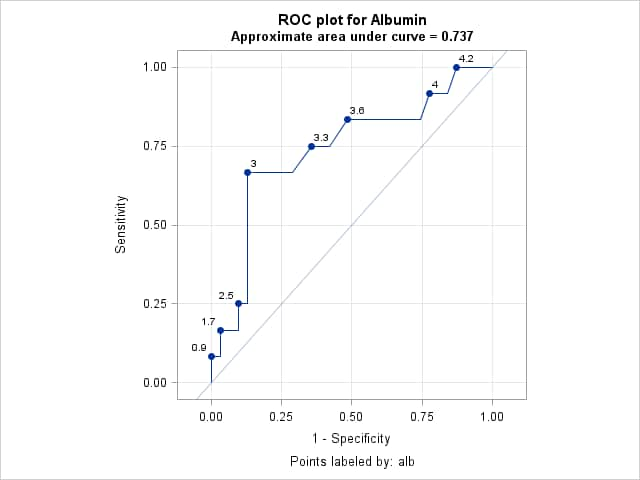
The following statements fit the model for the Albumin index. The ODS OUTPUT statement saves the table containing the area under the curve (AUC). The DATA _NULL_ step saves the AUC in a macro variable called ALBAREA. The ROCPLOT macro call plots the ROC curve and labels the cutpoints using the Albumin values. The THINSENS=0 and THINY=-1 options allow all cutpoints to be labeled.
     proc logistic data=roc plots(only)=roc(id=id);
       id alb;
       model popind(event="1") = alb / outroc=oralb;
       output out=albpred p=palb;
       ods output association=assoc;
       run;
     data _null_;
        set assoc;
        if label2="c" then call symput("albarea",cvalue2);
        run;
     title "ROC plot for Albumin";
     title2 "Approximate area under curve = &albarea";
     %rocplot(inpred=albpred, inroc=oralb, p=palb, id=alb, thinsens=0, thiny=-1)
     title2;
The following statements do the same as above for the K-G Score index.
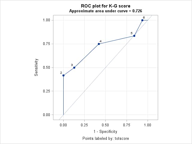
     proc logistic data=roc plots(only)=roc(id=id);
       id totscore;
       model popind(event="1") = totscore / outroc=ortots;
       output out=totspred p=ptots;
       ods output association=assoc;
       run;
     data _null_;
        set assoc;
        if label2="c" then call symput("totsarea",cvalue2);
        run;
     title "ROC plot for K-G score";
     title2 "Approximate area under curve = &totsarea";
     %rocplot(inpred=totspred, inroc=ortots, p=ptots, id=totscore, thinsens=0, thiny=-1)
     title2;
The following statements do the same as above for the Total Protein index.
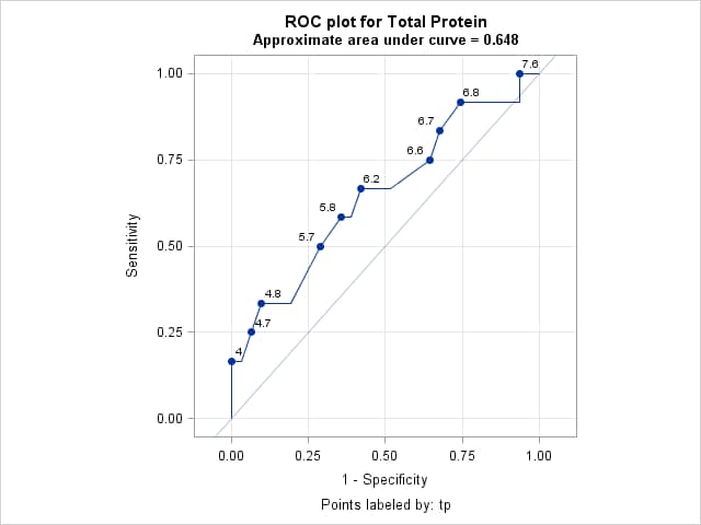
     proc logistic data=roc plots(only)=roc(id=id);
       id tp;
       model popind(event="1") = tp / outroc=ortp;
       output out=tppred p=ptp;
       ods output association=assoc;
       run;
     data _null_;
        set assoc;
        if label2="c" then call symput("tparea",cvalue2);
        run;
     title "ROC plot for Total Protein";
     title2 "Approximate area under curve = &tparea";
     %rocplot(inpred=tppred, inroc=ortp, p=ptp, id=tp, thinsens=0, thiny=-1)
     title2;
These statements produce a single comparative plot showing the ROC curves for all three indices and their AUC estimates.
     data allor;
        length Index $ 25;
        set oralb(in=alb) ortots(in=tots) ortp(in=tp);
        if alb then index="Albumin (&albarea)";
        else if tots then index="K-G Score (&totsarea)";
        else if tp then index="Total Protein (&tparea)";
        run;
     proc sgplot data=allor aspect=1;
        xaxis values=(0 to 1 by 0.25) grid offsetmin=.05 offsetmax=.05;
        yaxis values=(0 to 1 by 0.25) grid offsetmin=.05 offsetmax=.05;
        lineparm x=0 y=0 slope=1 / transparency=.7;
        series x=_1mspec_ y=_sensit_ / group=Index;
        run;
The following call of the ROC macro provides confidence intervals for the three ROC areas and compares the areas under the three ROC curves.
%roc(data=albpred tppred totspred, var=palb ptp ptots, response=popind) - RESULTS:
-
Following are the three ROC curves from the three ROCPLOT macro calls above.
Following is the comparative ROC plot showing all three ROC curves.
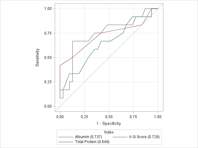
The results from the ROC macro call appear below. The AUC estimates for the three indices, along with standard errors and confidence intervals, are shown in the "ROC Curve Areas and 95% Confidence Intervals" table. The "Contrast Coefficients" table shows the default set of contrasts which provide pairwise comparisons among the three AUC estimates. Estimates of the pairwise differences, including confidence intervals on the differences, are provided in the "Tests and 95% Confidence Intervals for Contrast Rows" table. Finally, the "Contrast Test Results" table gives a test of the null hypothesis that the three AUCs are equal. The large p-value (p=0.2817) indicates insufficient evidence of any differences.
The ROC Macro
ROC Curve Areas and 95% Confidence Intervals ROC Area Std Error Confidence Limits palb 0.7366 0.0927 0.5549 0.9182 ptp 0.6478 0.1000 0.4518 0.8439 ptots 0.7258 0.1028 0.5243 0.9273
Contrast Coefficients palb ptp ptots Row1 1 -1 0 Row2 1 0 -1 Row3 0 1 -1
Tests and 95% Confidence Intervals for Contrast Rows Estimate Std Error Confidence Limits Chi-square Pr > ChiSq Row1 0.0887 0.0558 -0.0206 0.1981 2.5282 0.1118 Row2 0.0108 0.0953 -0.1761 0.1976 0.0127 0.9102 Row3 -0.0780 0.1046 -0.2830 0.1271 0.5554 0.4561
Contrast Test Results Chi-Square DF Pr > ChiSq 2.5340 2 0.2817
- EXAMPLE 2: Comparing three competing models
-
The data are from an example in Logistic Regression Using SAS:
Theory and Application, Second Edition by Paul Allison in which students
where asked if they would return a lost wallet and contents if found. The
response, WALLET, indicates if the wallet and contents would be returned
(WALLET=1) or kept (WALLET=0). Predictors are gender, whether in business
school, parental punishment at various ages, and parental explanation for
punishment.
Three models are fit and their ROC curve areas tested for equality. A significant finding is followed by pairwise comparisons.
   data wallet;
     input wallet male business punish explain @@;
     if wallet in (1,2) then wallet=0;
     if wallet=3 then wallet=1;
     datalines;
   2 0 0 2 0   3 0 0 1 1   3 1 0 1 1   2 0 1 1 1   3 1 0 1 1
   2 0 0 2 1   3 0 0 1 1   3 0 0 1 1   1 0 0 3 0   2 1 0 1 0
   3 0 0 1 1   3 0 0 1 1   3 0 1 1 1   1 0 1 2 0   3 0 1 2 1
   3 0 0 2 0   3 0 0 2 0   3 0 0 1 1   3 0 0 1 1   2 1 1 2 1
   1 1 0 1 1   3 1 1 1 1   3 0 0 1 1   3 0 0 1 1   3 0 0 1 1
   3 0 0 1 1   3 1 0 1 1   3 0 0 2 1   3 0 0 1 1   1 1 0 1 1
   3 0 0 1 1   3 0 0 1 1   2 1 1 1 0   3 1 1 1 1   3 1 1 3 1
   3 1 0 1 1   3 0 0 1 1   3 1 0 1 1   3 0 0 1 0   2 1 0 1 1
   3 1 0 1 1   3 0 0 1 0   3 0 0 1 1   3 0 0 1 1   1 0 0 1 0
   3 0 0 2 1   3 0 1 3 0   2 1 1 1 1   3 1 0 1 1   2 1 0 3 0
   2 0 1 1 1   3 1 0 2 0   3 0 0 1 1   3 1 1 1 1   3 0 0 1 1
   3 1 1 1 1   2 0 0 2 1   3 1 1 1 1   3 1 0 1 1   2 1 1 1 1
   3 1 0 1 1   3 0 0 1 1   3 0 0 1 1   2 1 1 1 1   3 0 0 1 1
   3 1 0 1 1   3 1 0 1 1   3 0 0 1 1   2 0 0 1 0   2 0 0 2 0
   3 0 0 1 1   3 1 0 1 1   3 0 0 1 1   3 0 0 1 1   2 1 0 1 1
   3 0 0 1 0   3 1 0 1 0   3 0 1 1 1   2 1 1 2 0   1 1 1 2 0
   3 0 0 2 1   3 1 1 1 0   3 0 0 2 1   3 1 0 1 0   2 1 0 2 0
   2 0 0 3 0   3 1 0 1 0   1 1 1 1 1   2 1 0 1 0   2 0 0 1 1
   1 1 1 3 0   2 1 1 3 1   1 1 0 2 0   3 0 0 2 1   1 0 1 3 0
   2 0 0 1 1   3 0 0 1 1   2 1 0 1 1   3 1 1 1 1   2 1 0 1 1
   2 1 0 2 0   3 0 0 3 1   1 1 1 1 1   1 0 0 3 0   2 1 0 1 1
   3 0 0 1 1   3 0 0 1 1   2 1 0 1 1   3 0 0 1 1   3 1 0 1 1
   3 1 0 1 1   3 0 0 1 0   1 1 1 3 0   3 1 1 1 1   3 0 0 1 1
   3 1 1 1 0   3 0 0 1 1   2 1 1 1 1   3 0 0 1 0   2 1 0 1 1
   3 1 0 1 1   1 0 1 1 1   1 1 1 3 1   3 0 1 1 0   1 1 0 2 0
   2 0 0 1 0   3 0 0 1 0   3 0 0 3 1   2 0 0 1 1   2 0 1 2 1
   2 1 0 3 0   3 1 0 1 1   3 0 0 1 1   3 1 0 1 1   3 0 0 2 0
   1 1 0 2 0   1 1 0 1 0   2 0 0 1 1   2 1 0 1 0   2 1 1 1 1
   3 1 0 2 0   3 1 0 3 1   3 0 0 1 1   3 0 0 1 0   3 0 1 2 1
   3 1 0 1 1   2 1 0 3 1   1 0 1 3 0   2 1 0 1 1   1 0 0 3 0
   3 0 0 1 1   1 1 1 2 1   3 0 0 1 1   3 1 0 1 1   2 1 1 1 0
   3 1 0 2 1   1 1 0 2 1   2 0 0 1 0   3 1 0 2 0   3 0 0 3 1
   1 1 0 1 1   3 0 0 1 1   3 0 0 1 1   3 1 1 2 1   2 1 0 2 1
   3 0 0 2 0   3 0 0 3 0   3 0 0 1 1   3 1 0 1 1   3 0 0 1 1
   3 1 0 1 0   2 1 0 1 1   2 1 0 1 1   2 1 0 1 0   3 1 0 3 1
   3 1 1 2 1   2 0 0 1 1   3 1 0 1 1   3 0 0 1 1   3 0 0 1 1
   3 0 0 2 0   2 1 0 1 1   3 0 0 1 1   3 1 0 1 1   3 1 1 1 1
   3 0 0 1 1   3 0 0 1 0   1 1 0 3 0   2 1 1 1 0   3 1 0 1 1
   3 1 0 1 1   3 1 1 1 1   2 1 0 1 1   3 0 0 1 1   2 1 0 1 1
   ;
   /* Fit three models to the Pr(return wallet) */
   proc logistic data=wallet;
     model wallet(event="1") = male business punish explain;
     output out=w1 xbeta=mbpe;
     run;

   proc logistic data=wallet;
     model wallet(event="1") = business punish explain;
     output out=w2 xbeta=bpe;
     run;

   proc logistic data=wallet;
     model wallet(event="1") = business punish ;
     output out=w3 xbeta=bp;
     run;

   /* Test equality of the three ROC curve areas. */
   %roc(data=w1 w2 w3,
        response=wallet,
        var=mbpe bpe bp)
The same analysis can be done in one PROC LOGISTIC step using ROC and ROCCONTRAST statements.
proc logistic data=wallet; mbpe: model wallet(event="1") = male business punish explain; roc 'bpe' business punish explain; roc 'bp' business punish; roccontrast / estimate=allpairs; run; - RESULTS:
- Following are the results from the %ROC macro. The overall p-value
(p=.0281) indicates that the three areas differ. The default pairwise
comparisons show that this difference is due to a significant difference
between the first and third models.
- EXAMPLE 3: Testing the area under the ROC curve
- You can test the null hypothesis that the area under an ROC curve is 0.5 by comparing the model of interest to an intercept-only model. The intercept-only model has area equal to 0.5, so the default contrast (1 -1) performs this test. These additional statements test the area of the last model in the previous example. The PROC LOGISTIC step fits the intercept-only model.
   proc logistic data=wallet;
     model wallet(event="1") =  ;
     output out=w4 xbeta=int;
     run;

   %roc(data=w3 w4,
        response=wallet,
        var=bp int)
The same analysis can be accomplished in PROC LOGISTIC using ROC and ROCCONTRAST statements as illustrated in this note.
- RESULTS:
- The test shows that the area under the ROC curve for this model is significantly different from 0.5 (p<0.0001).
The ROC Macro
ROC Curve Areas and 95% Confidence Intervals ROC Area Std Error Confidence Limits bp 0.6508 0.0379 0.5766 0.7250 int 0.5000 0.0000 0.5000 0.5000
Contrast Coefficients bp int Row1 1 -1
Tests and 95% Confidence Intervals for Contrast Rows Estimate Std Error Confidence Limits Chi-square Pr > ChiSq Row1 0.1508 0.0379 0.0766 0.2250 15.8648 <.0001
Contrast Test Results Chi-Square DF Pr > ChiSq 15.8648 1 <.0001
Right-click on the link below and select Save to save
the %ROC macro definition
to a file. It is recommended that you name the file
roc.sas.
| Type: | Sample |
| Topic: | Analytics ==> Regression SAS Reference ==> Procedures ==> LOGISTIC Analytics ==> Descriptive Statistics |
| Date Modified: | 2015-09-17 17:10:21 |
| Date Created: | 2005-01-13 15:03:44 |
Operating System and Release Information
| Product Family | Product | Host | SAS Release | |
| Starting | Ending | |||
| SAS System | SAS/STAT | Z64 | ||
| z/OS | ||||
| OpenVMS VAX | ||||
| Microsoft® Windows® for 64-Bit Itanium-based Systems | ||||
| Microsoft Windows Server 2003 Datacenter 64-bit Edition | ||||
| Microsoft Windows Server 2003 Enterprise 64-bit Edition | ||||
| Microsoft Windows XP 64-bit Edition | ||||
| Microsoft® Windows® for x64 | ||||
| OS/2 | ||||
| Microsoft Windows 8 Enterprise 32-bit | ||||
| Microsoft Windows 8 Enterprise x64 | ||||
| Microsoft Windows 8 Pro 32-bit | ||||
| Microsoft Windows 8 Pro x64 | ||||
| Microsoft Windows 8.1 Enterprise 32-bit | ||||
| Microsoft Windows 8.1 Enterprise x64 | ||||
| Microsoft Windows 8.1 Pro | ||||
| Microsoft Windows 8.1 Pro 32-bit | ||||
| Microsoft Windows 95/98 | ||||
| Microsoft Windows 2000 Advanced Server | ||||
| Microsoft Windows 2000 Datacenter Server | ||||
| Microsoft Windows 2000 Server | ||||
| Microsoft Windows 2000 Professional | ||||
| Microsoft Windows NT Workstation | ||||
| Microsoft Windows Server 2003 Datacenter Edition | ||||
| Microsoft Windows Server 2003 Enterprise Edition | ||||
| Microsoft Windows Server 2003 Standard Edition | ||||
| Microsoft Windows Server 2003 for x64 | ||||
| Microsoft Windows Server 2008 | ||||
| Microsoft Windows Server 2008 R2 | ||||
| Microsoft Windows Server 2008 for x64 | ||||
| Microsoft Windows Server 2012 Datacenter | ||||
| Microsoft Windows Server 2012 R2 Datacenter | ||||
| Microsoft Windows Server 2012 R2 Std | ||||
| Microsoft Windows Server 2012 Std | ||||
| Microsoft Windows XP Professional | ||||
| Windows 7 Enterprise 32 bit | ||||
| Windows 7 Enterprise x64 | ||||
| Windows 7 Home Premium 32 bit | ||||
| Windows 7 Home Premium x64 | ||||
| Windows 7 Professional 32 bit | ||||
| Windows 7 Professional x64 | ||||
| Windows 7 Ultimate 32 bit | ||||
| Windows 7 Ultimate x64 | ||||
| Windows Millennium Edition (Me) | ||||
| Windows Vista | ||||
| Windows Vista for x64 | ||||
| 64-bit Enabled AIX | ||||
| 64-bit Enabled HP-UX | ||||
| 64-bit Enabled Solaris | ||||
| ABI+ for Intel Architecture | ||||
| AIX | ||||
| HP-UX | ||||
| HP-UX IPF | ||||
| IRIX | ||||
| Linux | ||||
| Linux for x64 | ||||
| Linux on Itanium | ||||
| OpenVMS Alpha | ||||
| OpenVMS on HP Integrity | ||||
| Solaris | ||||
| Solaris for x64 | ||||
| Tru64 UNIX | ||||
| SAS System | SAS/IML | z/OS | ||
| Z64 | ||||
| OpenVMS VAX | ||||
| Microsoft® Windows® for 64-Bit Itanium-based Systems | ||||
| Microsoft Windows Server 2003 Datacenter 64-bit Edition | ||||
| Microsoft Windows Server 2003 Enterprise 64-bit Edition | ||||
| Microsoft Windows XP 64-bit Edition | ||||
| Microsoft® Windows® for x64 | ||||
| OS/2 | ||||
| Microsoft Windows 8 Enterprise 32-bit | ||||
| Microsoft Windows 8 Enterprise x64 | ||||
| Microsoft Windows 8 Pro 32-bit | ||||
| Microsoft Windows 8 Pro x64 | ||||
| Microsoft Windows 8.1 Enterprise 32-bit | ||||
| Microsoft Windows 8.1 Enterprise x64 | ||||
| Microsoft Windows 8.1 Pro | ||||
| Microsoft Windows 8.1 Pro 32-bit | ||||
| Microsoft Windows 95/98 | ||||
| Microsoft Windows 2000 Advanced Server | ||||
| Microsoft Windows 2000 Datacenter Server | ||||
| Microsoft Windows 2000 Server | ||||
| Microsoft Windows 2000 Professional | ||||
| Microsoft Windows NT Workstation | ||||
| Microsoft Windows Server 2003 Datacenter Edition | ||||
| Microsoft Windows Server 2003 Enterprise Edition | ||||
| Microsoft Windows Server 2003 Standard Edition | ||||
| Microsoft Windows Server 2003 for x64 | ||||
| Microsoft Windows Server 2008 | ||||
| Microsoft Windows Server 2008 R2 | ||||
| Microsoft Windows Server 2008 for x64 | ||||
| Microsoft Windows Server 2012 Datacenter | ||||
| Microsoft Windows Server 2012 R2 Datacenter | ||||
| Microsoft Windows Server 2012 R2 Std | ||||
| Microsoft Windows Server 2012 Std | ||||
| Microsoft Windows XP Professional | ||||
| Windows 7 Enterprise 32 bit | ||||
| Windows 7 Enterprise x64 | ||||
| Windows 7 Home Premium 32 bit | ||||
| Windows 7 Home Premium x64 | ||||
| Windows 7 Professional 32 bit | ||||
| Windows 7 Professional x64 | ||||
| Windows 7 Ultimate 32 bit | ||||
| Windows 7 Ultimate x64 | ||||
| Windows Millennium Edition (Me) | ||||
| Windows Vista | ||||
| Windows Vista for x64 | ||||
| 64-bit Enabled AIX | ||||
| 64-bit Enabled HP-UX | ||||
| 64-bit Enabled Solaris | ||||
| ABI+ for Intel Architecture | ||||
| AIX | ||||
| HP-UX | ||||
| HP-UX IPF | ||||
| IRIX | ||||
| Linux | ||||
| Linux for x64 | ||||
| Linux on Itanium | ||||
| OpenVMS Alpha | ||||
| OpenVMS on HP Integrity | ||||
| Solaris | ||||
| Solaris for x64 | ||||
| Tru64 UNIX | ||||