Usage Note 24188: Modeling rates and estimating rates and rate ratios (with confidence intervals)
 |  |  |
When the count of an event is observed over a period or amount of exposure, such as deaths per 100,000 individuals, traffic accidents per year, or injuries per person-year, it is called a rate. Unlike a proportion, which ranges from 0 to 1, a rate can have any nonnegative value, such as 4.2 deaths per 100,000 individuals or 65 accidents per year. The following is a log-linked model for a rate as a function of some predictor variables, x:
- log(μ/n) = x'β
where μ is the mean event count and n is the exposure. Note that this can be rewritten as
- log(μ)-log(n) = x'β
and it can be written as a model for log(μ) as
- log(μ) = log(n) + x'β
This is typically a Poisson or negative binomial model in which the additional term on the right-hand side, log(n), is called the offset. The offset is the log of the exposure, that is, the log of the rate denominator. It is a model term in which the associated parameter is fixed at 1. An offset can be added to a model in PROC GENMOD by specifying the OFFSET= option in the MODEL statement.
The following illustrates rate and rate ratio estimation in a Poisson model or negative binomial model. This note illustrates how differences, rather than ratios, of rates can be estimated. See this note for estimating and comparing rates in zero-inflated Poisson or negative binomial models.
Example: Modeling insurance claims rates
The insurance claim example in the "Getting Started" section of the GENMOD documentation illustrates fitting a Poisson model to the rate of insurance claims per policyholder, C/N, as a function of the size of car and age of the policyholder. The exposure variable, N, is the size of the policyholder population that has a given car size and policyholder age. The following statements fit the Poisson model
- log(μ/n) = β0 + β1·CARlarge + β2·CARmedium + β3·CARsmall + β4·AGE1 + β5·AGE2 ,
where β0 – β5 are the model parameters to be estimated, and CARlarge – AGE2 are 0,1-coded dummy variables created by the CLASS statement for the categorical Car and Age predictors.
      data insure;
         input n c car$ age;
         carnum=1;
         if car="medium" then carnum=2;
         if car="large" then carnum=3;
         ln = log(n);
         datalines;
         500   42  small  1
         1200  37  medium 1
         100    1  large  1
         400  101  small  2
         500   73  medium 2
         300   14  large  2
         ;

      proc genmod data=insure;
         class car age;
         model c = car age / dist=poisson link=log offset=ln;
         run;
Rate Estimates
The claim rates for the two AGE levels, averaged over the levels of CAR, are most easily obtained using the LSMEANS statement. The ILINK option applies the inverse link function to provide rate estimates. The CL option produces confidence intervals for the rates.
      proc genmod data=insure;
         class car age;
         model c = car age / dist=poisson link=log offset=ln;
         lsmeans age / ilink cl;
         run;
The estimated rate of claims for the AGE=1 population, 0.03156, appears in the Mean column. This is the estimated rate averaged over the levels of CAR. A confidence interval for this rate is (0.02395, 0.0416).
| ||||||||||||||||||||||||||||||||||||||||||||||||
Rate estimates at the six individual populations defined by the combinations of AGE and CAR levels can be obtained in three ways:
Using PROC PLM
Beginning in SAS® 9.4 TS1M1 you can use the NOOFFSET option in the SCORE statement of PROC PLM to compute rate estimates for the observations in the input data set or a data set of new observations. The STORE statement in PROC GENMOD saves the fitted model for later use by PROC PLM. The following statements compute and display predicted rates for the INSURE data set. The SOURCE= option reads the saved model. The SCORE statement in PROC PLM estimates rates, standard errors, and 95% confidence limits. The NOOFFSET option computes x'β so that rates rather than counts are estimated as shown in the first expression of the model above. The ILINK option applies the inverse of the link function. For this log-linked model, this means that the ILINK option computes exp(x'β), which is the rate.
      proc genmod data=insure;
         class car age;
         model c = car age / dist=poisson link=log offset=ln;
         store out=insmodel;
         run;

      proc plm source=insmodel;
         score data=insure out=inspred pred stderr lclm uclm / nooffset ilink;
         run;

      proc print label;
         id n c;
         run;
For the AGE=1, CAR=SMALL population, the estimated rate is 0.0716 with confidence interval (0.0553, 0.0927). This estimate applies specifically to AGE=1 in CAR=SMALL rather than being averaged over the CAR levels as done by the LSMEANS statement above.
|
Using the OUTPUT statement
The OUTPUT statement in PROC GENMOD can also be used to compute rate estimates. It can provide estimates for all observations in the input data set, and for new observations of interest if they are added to the original data set with missing response values. However, to get rate estimates and confidence intervals via the OUTPUT statement, some extra steps are needed because the P= option in the OUTPUT statement provides count estimates rather than rate estimates. The XBETA= option creates a variable containing the estimated log counts. This variable includes the offset, and as shown in the third expression of the model above, x'β plus the offset is the log count. The log rate is estimated by subtracting the offset contribution because, as shown in the first expression of the model, x'β alone estimates the log rate. The standard errors of the log counts are added to the OUT= data set by specifying the STDXBETA= option. The variances of the log rates and the log counts are the same because they differ only by an added constant (the offset). A large-sample confidence interval for the log rate is obtained by using the standard error of the log count. Point and interval estimates for the rates are obtained by exponentiating the point estimates and confidence limits for the log rates.
The following statements compute point estimates of the rates by subtracting the offset and exponentiating. Large-sample, 95% confidence limits are obtained by computing the limits around the log rate and then exponentiating those limits.
      proc genmod data=insure;
         class car age;
         model c = car age / dist=poisson link=log offset=ln;
         output out=out p=pcount xbeta=xb stdxbeta=std;
         run;

      data predrates;
         set out;
         obsrate=c/n;         /* observed rate */
         lograte=xb-ln;
         prate=exp(lograte);  /* predicted rate */
         lcl=exp(lograte-probit(.975)*std);
         ucl=exp(lograte+probit(.975)*std);
         keep n c car age prate lcl ucl;
         run;

      proc print data=predrates;
         id n c;
         run;
Note that the rate estimates and intervals match the above results from PROC PLM.
|
Using an ESTIMATE statement
You can also obtain a rate estimate for an individual population using the ESTIMATE statement. However, each ESTIMATE statement can estimate the rate for only one population, and you must identify that population by correctly specifying coefficients in the statement. This requires knowing how parameters are associated with predictor levels. Labeling in the "Analysis of Maximum Likelihood Parameter Estimates" table below makes this association clear. For example, the AGE=1, CAR=SMALL population is identified in the model by β0 + β3 + β4, that is the intercept plus the third (small) CAR parameter plus the first (1) AGE parameter.
| |||||||||||||||||||||||||||||||||||||||||||||||||||||||||||||||||||||||||||||||||
This provides the parameter coefficients needed in the ESTIMATE statement below.
      proc genmod data=insure;
         class car age;
         model c = car age / dist=poisson link=log offset=ln;
         estimate "Rate: age=1, small" intercept 1 age 1 0 car 0 0 1;
         run;
The sum of these three parameters yields the "L'Beta Estimate," -2.6367, which is the estimated log rate for this population. The estimated rate, 0.0716 (or about 7 claims in 100 policyholders), is labeled as the "Mean Estimate" NOTE with a confidence interval of (0.0553, 0.0927) or about 5.5 to 9.3 claims per 100 policyholders. This is the same result found by the previous two methods.
| |||||||||||||||||||||||||||||||||||||
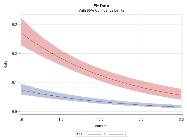
Plotting the rate model
A plot of the fitted rate model can be produced using the EFFECTPLOT statement in PROC GENMOD. Using the CARNUM variable in the MODEL statement treats car size as a continuous predictor rather than categorical. These statements fit the new model and plot the estimated rates as a function of car size. The MOFF option removes the offset so that estimated rates are plotted rather than estimated counts. The CLM option includes confidence bands for the estimated rate curves.
      proc genmod data=insure;
         class age;
         model c = carnum age / dist=poisson link=log offset=ln;
         effectplot / clm moff;
         run;
|
Note that the EFFECTPLOT statement above is equivalent to the following statement:
effectplot slicefit(x=carnum sliceby=age) / clm moff;
Rate Ratio Estimates
The ESTIMATE and LSMEANS statements can be used to estimate the ratio of two population rates. The LSMEANS statement is the easiest way to produce rate ratio estimates. If you are interested in estimating a difference in rates rather than ratio, see this note.
Using the LSMEANS statement
A comparison of AGE rates can be accomplished most easily using the LSMEANS statement since it is not necessary to define the specific linear combination of model parameters. As before, the LSMEANS statement below requests estimation of LS-means for each AGE level. The addition of the DIFF option provides all pairwise differences among the AGE levels. The EXP option is also added to exponentiate the LS-mean estimates and the difference estimates. This results in the estimate of the AGE rate ratio.
      proc genmod data=insure;
         class car age;
         model c = car age / dist=poisson link=log offset=ln;
         lsmeans age / ilink diff exp cl;
         run;
The estimated ratio of the AGE=1 rate to the AGE=2 rate is 0.2672 with a confidence interval of (0.2047, 0.3487). The rate ratio is significantly different from one (p<0.0001).
| ||||||||||||||||||||||||||||||||||||
Using the ESTIMATE statement
The ESTIMATE statement requires the coefficients of the linear combination of model parameters that define the desired quantity. Under the fitted model, the difference of the log rates in the two age levels for small cars is
log(μ1/n1) - log(μ2/n2) = (β0+β3+β4) - (β0+β3+β5) = 1·β4 + (-1)·β5
The coefficients 1 and -1 are used in the ESTIMATE statement below to estimate this difference. Because β5 is set to zero by the model parameterization, the difference is simply β4. The same result occurs for medium and large cars. Since the difference in logs is the log of the ratio
log(μ1/n1) - log(μ2/n2) = log[(μ1/n1) / (μ2/n2)] ,
β4 is the log rate ratio that compares AGE=1 to AGE=2 for any car size, and exp(β4) is the rate ratio comparing AGE 1 and 2. A test of β4=0 is provided in the "Analysis of Maximum Likelihood Parameter Estimates" table. Note that testing β4=0 is equivalent to testing exp(β4)=1.
Because the difference in log rates is simply a linear combination of model parameters as shown above, the ESTIMATE statement can provide point and interval estimates of it.
      proc genmod data=insure;
         class car age;
         model c = car age / dist=poisson link=log offset=ln;
         estimate "Age Rate Ratio" age 1 -1;
         run;
The "L'Beta Estimate" from the ESTIMATE statement above estimates the difference in the log rates (or log rate ratio), -1.3199, for the two AGE levels and is equivalent to the β4 parameter estimate. The "Mean Estimate" results from applying the inverse link function. The mean estimate is the estimated rate ratio, 0.2672, which is the same estimate provided by the DIFF and EXP options in the LSMEANS statement. A test that the "L'Beta Estimate" equals zero (or equivalently that the rate ratio equals one) is also provided and matches the test of the β4 parameter in the "Analysis of Maximum Likelihood Parameter Estimates" table shown above.
| |||||||||||||||||||||||||||||||||||||
You can estimate and test custom rate ratios by using the appropriate coefficients in the ESTIMATE statement. See Examples of Writing CONTRAST and ESTIMATE Statements for more information about determining proper coefficients for custom contrasts.
_____
NOTE: In releases prior to SAS 9.2, the EXP option is needed in the ESTIMATE statement to exponentiate the estimated linear combination resulting in a rate ratio estimate. Beginning in SAS 9.2, the EXP option is no longer needed since estimates of the contrast applying the inverse link function (labeled "Mean") are provided by default.
Operating System and Release Information
| Product Family | Product | System | SAS Release | |
| Reported | Fixed* | |||
| SAS System | SAS/STAT | All | n/a | |
| Type: | Usage Note |
| Priority: | low |
| Topic: | SAS Reference ==> Procedures ==> GENMOD Analytics ==> Categorical Data Analysis Analytics ==> Regression SAS Reference ==> Procedures ==> PLM |
| Date Modified: | 2015-01-12 13:54:28 |
| Date Created: | 2004-10-22 15:07:07 |