Usage Note 24170: Sensitivity, specificity, positive and negative predictive values, and other 2x2 table statistics
 |  |  |
There are many common statistics defined for 2×2 tables. Some statistics are available in PROC FREQ. Others can be computed as discussed and illustrated below.
The following hypothetical data assume that subjects were observed to exhibit the response (such as a disease) or not. Subjects also tested either positive (Test=1) or negative (Test=0) on a prognostic test for the response. Results from all subjects can be summarized in a 2×2 table.
These statements read in the cell counts of the table and use PROC FREQ to display the table. PROC SORT orders the row and column variables so that 1 appears before 0. The ORDER=DATA option in PROC FREQ orders the table according to the order found in the sorted data set. As a result, the 1 levels appear before the 0 levels, putting Test=1, Response=1 in the upper-left (1,1) cell of the table:
      data FatComp;
         input Test Response Count;
         datalines;
         0 0  6
         0 1  2
         1 0  4
         1 1 11
         ;
      proc sort data=FatComp;
         by descending Test descending Response;
         run;
      proc freq data=FatComp order=data;
         weight Count;
         tables Test*Response / senspec;
         run;
Point estimates for sensitivity, specificity, positive predictive value (PPV), negative predictive value (NPV), false positive probability, and false negative probability are row or column percentages of the 2×2 tableNote. Beginning in SAS® 9.4M6 (TS1M6), point estimates and confidence intervals for sensitivity, specificity, PPV, and NPV are available in PROC FREQ (and in PROC SURVEYFREQ) with the SENSPEC option in the TABLES statement as shown above. In earlier releases, estimates, confidence intervals, and tests of the above statistics can be obtained either by using PROC FREQ on subtables or by using a modeling procedure to estimate the statistics. This is illustrated below.
A common estimate (meta-analysis) of any of these four statistics, computed using the data from multiple studies, can be obtained as shown in SAS Note 71101.
Here are the results from PROC FREQ, with sensitivity, specificity, positive predictive value, negative predictive value, false positive probability, and false negative probability indicated by matching colors:
|
The FREQ Procedure
|
||||||||||||||||||||||||||||||||||||||||||||||||||||||||||||
The estimates highlighted above are repeated in the results from the SENSPEC option along with their standard error estimates and confidence intervals:
|
||||||||||||||||||||||||||||||
All statistics discussed in this note are defined as follows, assuming that the table is arranged as shown with Response levels as the columns and Test levels as the rows and with Test=1, Response=1 in the (1,1) cell of the table.
- The sensitivity (also called recall or true positive rate, TPR)Note is the proportion of true positive responders (Response=1) that have a positive test result (Test=1). This is the proportion of the first column that is in the (1,1) cell, 11/13 = 0.8462, and is given as the column percentage (Col Pct) for the (1,1) cell (84.62%).
- The specificity (also called the true negative rate, TNR)Note is the proportion of true negative responders (Response=0) that have a negative test result (Test=0), 6/10 = 0.6, and is the column percentage for the (0,0) cell.
- The positive predictive value (PPV) (also called precision)Note is the proportion of positive test results that are true positive responders, 11/15 = 0.7333, the row percentage (Row Pct) for the (1,1) cell. Using Bayes' theorem, PPV can be defined to be a function of the overall probability of true response.
- The negative predictive value (NPV) is the proportion of negative test results that are true negative responders, 6/8 = 0.75, the row percentage for the (0,0) cell. Like PPV, NPV can be defined as a function of the overall true response probability by using Bayes' theorem.
- The definition of the false positive probability or rate (FPR) is not universal. Some define it as the proportion of true negative responders that have a positive test result (4/10 = 0.4). This is sometimes called the false discovery rate, FDR. Others define it as the proportion of positive test results that are true negative responders (4/15 = 0.2667). Both focus on the (1,0) cell, but the former is the column percentage while the latter is the row percentage.
- Similarly, the definition of the false negative probability is sometimes the proportion of true positive responders that have a negative test result (2/13 = 0.1538). This is sometimes called the false omission rate, FOR. It is sometimes defined as the proportion of negative test results that are true positive responders (2/8 = 0.25). Both focus on the (0,1) cell, but the former is the column percentage while the latter is the row percentage.
- F1Note is a combination of PPV and sensitivity (TPR), or precision and recall. It is their harmonic mean and is computed as 2*(PPV*TPR)/(PPV+TPR). For the table above, F1 = 0.7857.
- The accuracy or correct classification rate is the proportion of observations for which the test result and actual response agree: (11 + 6)/23 = 0.7391.
- The lift is the ratio of the positive response proportion in a test level to the overall proportion of positive responders. For Test=1, Lift+ = (11/15)/(13/23) = 1.2974. For Test=0, Lift- = (2/8)/(13/23) = 0.4423.
- The likelihood ratio of a positive test result (denoted LR+) is sensitivity divided by 1-specificity = (11/13)/[1-(6/10)] = 2.1154. The likelihood ratio of a negative test result (denoted LR-) is 1-sensitivity divided by specificity = [1-(11/13)]/(6/10) = 0.2564. For more on the computation and interpretation of the likelihood ratio statistics, see SAS KB0044428.
- The attributable risk (AR) (or fraction) is the fraction of event proportion in the exposed population that is attributable to exposure. Computed as AR = (Re-Ru)/Re, where Re is the risk in the exposed group and Ru is the risk in the unexposed group. For the above example, AR = ((11/15)-(2/8))/(11/15) = 0.659. It can be estimated using the METHOD=MH(AF) and STAT=RISK options in PROC STDRATE. See also SAS Note 63471, which discusses adjusting for covariates.
- The population attributable risk (PAR) (or fraction) is the reduction in the event proportion in the population attributable to avoiding the risk factor. Computed as PAR = (R-Ru)/R, where R is the overall risk in the combined exposed and unexposed groups. For the above example, PAR = ((13/23)-(2/8))/(13/23) = 0.558. Similarly to AR, it can be estimated using the METHOD=MH(AF) and STAT=RISK options in PROC STDRATE. See also SAS Note 63471, which discusses adjusting for covariates.
- The number needed to treat is the number of subjects that need to receive a treatment in order to obtain one more beneficial response. It is computed as the reciprocal of the risk difference: 1/((11/15)-(2/8)) = 2.0690.
Using PROC NLMIXED to Estimate and Test All Statistics
One way to obtain estimates of all of the above statistics, along with their standard errors (computed using the delta method) and large-sample confidence intervals, is to use PROC NLMIXED. This is done by fitting a saturated Poisson model that has one parameter in the model for each cell of the table. Then each statistic can be estimated by specifying its formula in an ESTIMATE statement. This is illustrated in the following NLMIXED step that produces the estimates shown above. A similar approach can be used to compare statistics computed in two or more independent tables as discussed in SAS KB0044428.
Note that each ESTIMATE statement includes a large-sample test of the null hypothesis that the specified function equals 0. For ratios, such as the lift and likelihood ratio statistics, where it is of interest to test their equality to 1 rather than 0, a second ESTIMATE statement is used that subtracts 1 from the function to test that the ratio equals 1:
    proc nlmixed data=FatComp df=1e8;
       mu=exp(t0r0*(test=0 and response=0) + t0r1*(test=0 and response=1) +
              t1r0*(test=1 and response=0) + t1r1*(test=1 and response=1));
       model count ~ poisson(mu);

       /* Cell Counts and Margins */
       n11=exp(t1r1); n10=exp(t1r0); n01=exp(t0r1); n00=exp(t0r0);
       /* Test margins and Response margins */
       t1=n11+n10; t0=n01+n00;
       r1=n11+n01; r0=n10+n00;
       total=n11+n10+n01+n00;

       /* Statistics */
       estimate 'Sensitivity/TPR/Recall' n11/r1;
       estimate 'Specificity/TNR' n00/r0;
       estimate 'PPV/Precision' n11/t1;
       estimate 'NPV' n00/t0;
       estimate 'FPR/FDR' n10/t1;
       estimate 'FPR' n10/r0;
       estimate 'FNR/FOR' n01/t0;
       estimate 'FNR' n01/r1;
       estimate 'Accuracy' (n00+n11)/total;
       estimate 'Test Lift+ = 1' (n11/t1)/(r1/total)-1;
       estimate 'Estimate Lift-' (n01/t0)/(r1/total);
       estimate 'Test Lift- = 1' (n01/t0)/(r1/total)-1;
       estimate 'Estimate LR+' (n11/r1)/(1-n00/r0);
       estimate 'Test LR+ = 1' (n11/r1)/(1-n00/r0)-1;
       estimate 'Estimate LR-' (1-n11/r1)/(n00/r0);
       estimate 'Test LR- = 1' (1-n11/r1)/(n00/r0)-1;
       estimate 'AR' ((n11/t1)-(n01/t0))/(n11/t1);
       estimate 'PAR' ((r1/total)-(n01/t0))/(r1/total);
       estimate 'NNT' 1/((n11/t1)-(n01/t0));
       estimate 'F1' 2*(((n11/t1)*(n11/r1))/((n11/t1)+(n11/r1)));
       run;
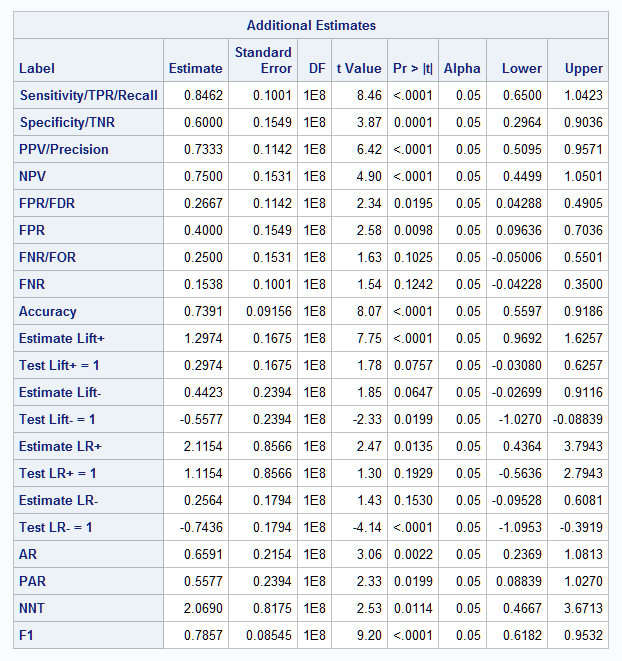
Here are the results from the ESTIMATE statements in PROC NLMIXED, including point estimates, tests, and confidence intervals for the statistics. For each of the lift and LR statistics, the results from the first ESTIMATE statement provide the point estimate and confidence interval. The results from the second ESTIMATE statement provide a test that the ratio function defining the statistic equals 1 – the Estimate and confidence limit values can be ignored:
 |
Other Methods to Estimate and Test the Statistics
Alternatively, the BINOMIAL option in the TABLES statement of PROC FREQ can be used to obtain asymptotic and exact confidence intervals and an asymptotic test that the proportion equals 0.5 (by default). The BINOMIAL option in the EXACT statement provides all of this plus an exact test of the proportion. You can test against a null value other than 0.5 by specifying P=value in parentheses after the BINOMIAL option. For example, BINOMIAL(P=0.75) tests against the null value of 0.75.
The following statements estimate and test each of the first six statistics as indicated in the TITLE statements. The WHERE statement is used to select the proper row or column for the statistic in each case. The use of LEVEL= in the BINOMIAL option selects the level of TEST or RESPONSE whose probability is estimated:
      title 'Sensitivity/TPR/Recall';
      proc freq data=FatComp;
         where Response=1;
         weight Count;
         tables Test / binomial(level="1");
         exact binomial;
         run;

      title 'Specificity/TNR';
      proc freq data=FatComp;
         where Response=0;
         weight Count;
         tables Test / binomial(level="0");
         exact binomial;
         run;

      title 'Positive predictive value/Precision';
      proc freq data=FatComp;
         where Test=1;
         weight Count;
         tables Response / binomial(level="1");
         exact binomial;
         run;

      title 'Negative predictive value';
      proc freq data=FatComp;
         where Test=0;
         weight Count;
         tables Response / binomial(level="0");
         exact binomial;
         run;

      title 'False Positive Probability/FDR (Col)';
      proc freq data=FatComp;
         where Response=0;
         weight Count;
         tables Test / binomial(level="1");
         exact binomial;
         run;

      title 'False Positive Probability (Row)';
      proc freq data=FatComp;
         where Test=1;
         weight Count;
         tables Response / binomial(level="0");
         exact binomial;
         run;

      title 'False Negative Probability/FOR (Col)';
      proc freq data=FatComp;
         where Response=1;
         weight Count;
         tables Test / binomial(level="0");
         exact binomial;
         run;

      title 'False Negative Probability (Row)';
      proc freq data=FatComp;
         where Test=0;
         weight Count;
         tables Response / binomial(level="1");
         exact binomial;
         run;
Here are the results for sensitivity. Note that the estimate, 0.8462, is the same as shown above. An asymptotic confidence interval (0.65, 1) and an exact confidence interval (0.55, 0.98) for sensitivity are given. Also provided are asymptotic and exact one- and two-sided tests of the null hypothesis that sensitivity = 0.5:
The FREQ Procedure
Sample Size = 13
|
||||||||||||||||||||||||||||||||||||||||||||||||||||||
The accuracy can be computed by creating a binary variable (ACC), indicating whether test and response agree in each observation. As above, the BINOMIAL option in the TABLES and EXACT statements can be used to obtain asymptotic and exact tests and confidence intervals:
      data acc;
         set FatComp;
         acc = (test = response);
         run;
      proc freq;
         weight count;
         tables acc / binomial(level="1");
         exact binomial;
         run;
The accuracy is again found to be 0.7391 with a confidence interval of (0.56, 0.92). Asymptotic and exact tests of the null hypothesis that accuracy = 0.5 are similar and significant:
|
|||||||||||||||||||||||||||||||||||||||||||||||||||||
The lift values can be estimated in PROC GENMOD by fitting a log-linked binomial model to the data. This models the log of the positive response probabilities in the Test levels. By using the log of the overall probability of positive response as the offset, the log of the lift is modeled. The LSMEANS statement with the ILINK and CL options estimates the lift and provides a confidence interval and a test that the lift equals one:
data lift;
   set FatComp;
   off=log(13/23);
   run;
proc genmod data=lift descending;
   freq count;
   class test;
   model response=test / dist=binomial link=log offset=off;
   lsmeans test / ilink cl;
   run;
In the results from the LSMEANS statement, the Estimate column contains the log lift estimates. The lift estimates appear in the Mean column and the confidence limits are in the Lower Mean and Upper Mean columns. The p-value for the test that the lift equals one is in the Pr>|z| column:
|
||||||||||||||||||||||||||||||||||||||||||||||||
The likelihood ratios, LR+ and LR-, can be easily computed from the sensitivity and specificity as described above. Since they can also be seen as nonlinear functions (ratios) of model parameters, they can be computed using the NLEST/NLEstimate macro (SAS Note 58775), which provides a large sample confidence interval for each. PROC GENMOD is used to fit this linear probability model with TEST as the response and RESPONSE as a categorical predictor:
Pr(TEST=1) = β0RESPONSE0 + β1RESPONSE1 ,
where RESPONSE0 equals 1 if RESPONSE=0, and equals 0 otherwise, and RESPONSE1 equals 1 if RESPONSE=1, and equals 0 otherwise. Under this model, β1 is the sensitivity and β0 is 1-specificity. When fitting the model in PROC GENMOD, include the STORE statement to save the model. Create a data set with an observation for each function to be estimated. See the description of the NLEST macro for details:
      proc genmod data=FatComp descending;
         freq count;
         class response test;
         model test = response / dist=binomial link=identity noint;
         store genfit;
         run;
      data fd;
         length label f $32767;
         infile datalines delimiter=',';
         input label f;
         datalines;
      LR+, b_p2/b_p1
      LR-, (1-b_p2)/(1-b_p1)
      ;
      %nlest(instore=genfit, fdata=fd, null=1)
The point estimates of LR+ and LR- agree with the computations above (2.1154 and 0.2564 respectively). The 95% large sample confidence interval for LR+ is (0.4364, 3.7943) and for LR- is (-0.0926, 0.6081). A test that each ratio equals 1 is provided by specifying null=1 in the NLEST macro call. These results match those from the PROC NLMIXED analysis above:
 |
Computation of the attributable risk and population attributable risk (PAR) requires a data set of event counts and total counts for each population. In the above table, the Test levels are the populations and Response=1 is the event of interest. The TestCnts data set below contains the event counts (Count) and total counts (Total) for each Test population. Note that the population representing presence of the risk factor (Test=1) appears first. PROC STDRATE estimates the two risks by specifying the METHOD=MH(AF) and STAT=RISK options. In the POPULATION statement, the Test variable is identified as the GROUP= variable indicating the populations. The GROUP(EXPOSED="1")=Test option specifies that the Test=1 group is the exposed group. The event and total count variables are specified in the EVENT= and TOTAL= options:
      data TestCnts;
         input Test Count Total;
         datalines;
      1 11 15
      0  2  8
      ;

      proc stdrate data=TestCnts method=mh(af) stat=risk;
         population group(exposed="1")=Test event=Count total=Total;
         run;
The final table from PROC STDRATE presents the two risk estimates and their confidence intervals:
|
||||||||||||||||
See also the example titled "Computing Attributable Fraction Estimates" in the STDRATE documentation (SAS Note 22930) and SAS Note 63471, which discusses adjusting the estimates for covariates.
The number needed to treat (NNT) can be estimated in various ways. One way is shown above using PROC NLMIXED. Since NNT is equal to the reciprocal of the risk difference, one way is to obtain the risk difference estimate and standard error from PROC FREQ and then use the delta method to obtain a standard error and confidence limits for NNT. Another modeling approach fits a logistic model and estimates the appropriate nonlinear function of the logistic model parameters.
The PROC FREQ approach is shown below. Begin by obtaining the risk difference and its standard error from PROC FREQ. Since the table is arranged so that Test=1, Response=1 appears in the upper-left (1,1) cell of the table, the Column 1 risk difference is needed. The following ODS OUTPUT statement saves the Column 1 risk difference in a data set:
      proc freq data=FatComp order=data;
         weight Count;
         tables Test*Response / riskdiff;
         ods output RiskdiffCol1=rd;
         run;
Note that the positive response probability for those positive on the prognostic test (TEST=1) is 0.7333 and is 0.25 for those negative on the test (TEST=0). The risk difference is then 0.7333 - 0.25 = 0.4833:
|
|||||||||||||||||||||||||||||||||||||||||||||||||
The following statements compute the estimate of the NNT and use the estimator obtained from the delta method to provide a (1-α)100% confidence interval:
      data nnt;
         set rd;
         where Row="Difference";
         alpha=.05;
         NNT=1/risk;
         NNT_SE=ase/risk**2; *by delta method;
         LCL=nnt-probit(1-alpha/2)*nnt_se;
         UCL=nnt+probit(1-alpha/2)*nnt_se;
         run;

      proc print;
         id table;
         var NNT NNT_SE LCL UCL;
         run;
The results show that a little over two subjects (2.0690) need to be treated, on average, to obtain one more positive response. A 95% large sample confidence interval for the NNT is (0.4666, 3.6713):
|
The following statements fit a logistic model to the FatComp data and store the fitted model in an item store named Log. Similar to the example in SAS Note 37228, the risk at each Test level is written in terms of the model parameters and the reciprocal of the difference is specified in the f= option of the NLEST macro for estimation. The parameters are referred to using names as described in the documentation for the NLEST/NLEstimate macro (SAS Note 58775). The macro provides an estimate of the NNT and a large sample confidence interval:
	proc logistic data=FatComp;
	   freq Count;
	   model Response(event="1")=Test;
	   store Log;
	   run;
	%nlest(instore=Log, label=NNT, f=1/(logistic(B_p1+B_p2)-logistic(B_p1)))
The results match those from the PROC FREQ and PROC NLMIXED approaches above.
________
Note: Many of these statistics are used to evaluate the performance of a model or classifier on a binary (event/nonevent) response, which assigns a probability of being the event to each observation in the input data set. By selecting a cutoff (or threshold) between 0 and 1, it can be compared against the predicted event probabilities and every observation can be classified as either a predicted event or a predicted nonevent by the model or classifier. A 2x2 table of predicted versus actual response levels can then be constructed and these statistics can be computed. In this way, the statistics can be computed for each cutoff over a range of values. Using this method, the sensitivity and 1-specificity pairs associated with the various selected cutoffs can be plotted to produce the ROC (Receiver Operating Characteristic) curve. Similarly, the precision and recall pairs can be plotted to produce the precision-recall (PR) curve. The ROC curve, and the area under it, can be produced by PROC LOGISTIC. See "ROC (Receiver Operating Characteristic) curve" in SAS Note 30333. The PR curve, and the area under it, can be produced by the PRcurve macro (SAS Note 68077).
Operating System and Release Information
| Product Family | Product | System | SAS Release | |
| Reported | Fixed* | |||
| SAS System | SAS/STAT | All | n/a | |
| Type: | Usage Note |
| Priority: | low |
| Topic: | SAS Reference ==> Procedures ==> FREQ Analytics ==> Exact Methods Analytics ==> Categorical Data Analysis Analytics ==> Descriptive Statistics SAS Reference ==> Procedures ==> STDRATE SAS Reference ==> Procedures ==> GENMOD SAS Reference ==> Macro SAS Reference ==> Procedures ==> SURVEYFREQ SAS Reference ==> Procedures ==> NLMIXED |
| Date Modified: | 2025-02-25 09:25:22 |
| Date Created: | 2004-09-23 15:44:42 |