Usage Note 22627: Missing inverse confidence limits from the INVERSECL option or the IPPPLOT statement in PROC PROBIT
 |  |  |
If the parameter estimate of the first continuous (i.e. not in the CLASS statement) predictor variable is not strongly significant, some limits shown in the table of inverse confidence limits may be missing and the inverse confidence bands may not appear in the plot produced by the IPPPLOT statement.
Notice in this example that the slope of the predictor, X, is not significantly different from zero.
| Analysis of Parameter Estimates | |||||||
| Parameter | DF | Estimate | Standard Error | 95% Confidence Limits | Chi-Square | Pr > ChiSq | |
| Intercept | 1 | 0.2012 | 0.1922 | -0.1754 | 0.5779 | 1.10 | 0.2950 |
| x | 1 | -0.0343 | 0.0310 | -0.0950 | 0.0264 | 1.23 | 0.2680 |
As a result of the near-zero slope, the inverse confidence limits do not exist and are displayed as missing in the results of the INVERSECL option:
| Probit Analysis on x | |||
| Probability | x | 95% Fiducial Limits | |
| 0.01 | 73.717 | . | . |
| 0.02 | 65.767 | . | . |
| 0.03 | 60.723 | . | . |
| 0.04 | 56.928 | . | . |
| 0.05 | 53.842 | . | . |
| 0.06 | 51.214 | . | . |
| 0.07 | 48.911 | . | . |
| 0.08 | 46.848 | . | . |
| 0.09 | 44.973 | . | . |
| 0.10 | 43.246 | . | . |
| 0.15 | 36.097 | . | . |
| 0.20 | 30.415 | . | . |
| 0.25 | 25.541 | . | . |
| 0.30 | 21.164 | . | . |
| 0.35 | 17.107 | . | . |
| 0.40 | 13.258 | . | . |
| 0.45 | 9.534 | . | . |
| 0.50 | 5.869 | . | . |
| 0.55 | 2.204 | . | . |
| 0.60 | -1.520 | . | . |
| 0.65 | -5.369 | . | . |
| 0.70 | -9.425 | . | . |
| 0.75 | -13.802 | . | . |
| 0.80 | -18.677 | . | . |
| 0.85 | -24.358 | . | . |
| 0.90 | -31.507 | . | . |
| 0.91 | -33.234 | . | . |
| 0.92 | -35.110 | . | . |
| 0.93 | -37.172 | . | . |
| 0.94 | -39.476 | . | . |
| 0.95 | -42.103 | . | . |
| 0.96 | -45.190 | . | . |
| 0.97 | -48.984 | . | . |
| 0.98 | -54.028 | . | . |
| 0.99 | -61.979 | . | . |
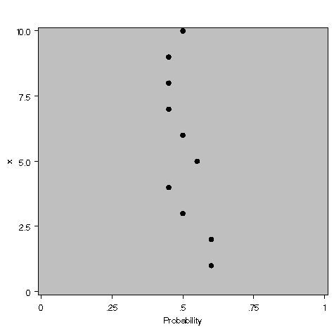
Also, no limits are displayed in the inverse predicted probability plot from the IPPPLOT statement:

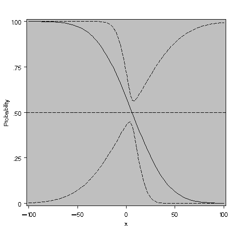
Using the PREDPPLOT statement, you can get an idea of what the problem is. Note that the range in this plot (-100 to 100) is greatly expanded beyond the range of the observed predictor (1 to 10 in this example) so that the characteristic shape of the probit model can be seen.

The plot for this model shows the fitted curve and confidence limits for the predicted values. Keep in mind that you're trying to get a confidence interval on the predictor variable that would generate a given response probability. While the inverse confidence limits are not just the inverse of the confidence limits for the predicted values, the plot is instructive. Notice that a reference line drawn at a response probability (such as 0.5 as shown) does not intersect the confidence bands on the predicted probabilities. This suggests that the inverse confidence limits do not exist.
Here is an example in which the slope of the predictor is significant and all limits exist:
| Analysis of Parameter Estimates | |||||||
| Parameter | DF | Estimate | Standard Error | 95% Confidence Limits | Chi-Square | Pr > ChiSq | |
| Intercept | 1 | -1.3788 | 0.2326 | -1.8347 | -0.9228 | 35.12 | <.0001 |
| x | 1 | 0.1313 | 0.0351 | 0.0625 | 0.2002 | 13.97 | 0.0002 |
As a result of the significant slope, all inverse confidence limits exist and are displayed by the INVERSECL option:
| Probit Analysis on x | |||
| Probability | x | 95% Fiducial Limits | |
| 0.01 | -7.2153 | -21.9487 | -2.5141 |
| 0.02 | -5.1396 | -17.6120 | -1.1247 |
| 0.03 | -3.8227 | -14.8663 | -0.2373 |
| 0.04 | -2.8320 | -12.8053 | 0.4346 |
| 0.05 | -2.0261 | -11.1326 | 0.9850 |
| 0.06 | -1.3402 | -9.7123 | 1.4570 |
| 0.07 | -0.7388 | -8.4705 | 1.8742 |
| 0.08 | -0.2003 | -7.3619 | 2.2511 |
| 0.09 | 0.2894 | -6.3572 | 2.5974 |
| 0.10 | 0.7402 | -5.4360 | 2.9198 |
| 0.15 | 2.6067 | -1.6817 | 4.3145 |
| 0.20 | 4.0900 | 1.1579 | 5.5670 |
| 0.25 | 5.3627 | 3.3421 | 6.8935 |
| 0.30 | 6.5055 | 4.9436 | 8.4447 |
| 0.35 | 7.5645 | 6.1049 | 10.2049 |
| 0.40 | 8.5694 | 7.0176 | 12.0644 |
| 0.45 | 9.5417 | 7.8051 | 13.9591 |
| 0.50 | 10.4985 | 8.5297 | 15.8741 |
| 0.55 | 11.4554 | 9.2251 | 17.8183 |
| 0.60 | 12.4276 | 9.9133 | 19.8122 |
| 0.65 | 13.4325 | 10.6118 | 21.8859 |
| 0.70 | 14.4915 | 11.3385 | 24.0807 |
| 0.75 | 15.6344 | 12.1152 | 26.4567 |
| 0.80 | 16.9070 | 12.9737 | 29.1090 |
| 0.85 | 18.3904 | 13.9684 | 32.2064 |
| 0.90 | 20.2568 | 15.2137 | 36.1100 |
| 0.91 | 20.7076 | 15.5137 | 37.0536 |
| 0.92 | 21.1974 | 15.8393 | 38.0790 |
| 0.93 | 21.7359 | 16.1971 | 39.2068 |
| 0.94 | 22.3373 | 16.5963 | 40.4667 |
| 0.95 | 23.0232 | 17.0511 | 41.9040 |
| 0.96 | 23.8290 | 17.5851 | 43.5931 |
| 0.97 | 24.8197 | 18.2409 | 45.6703 |
| 0.98 | 26.1367 | 19.1118 | 48.4325 |
| 0.99 | 28.2124 | 20.4828 | 52.7876 |
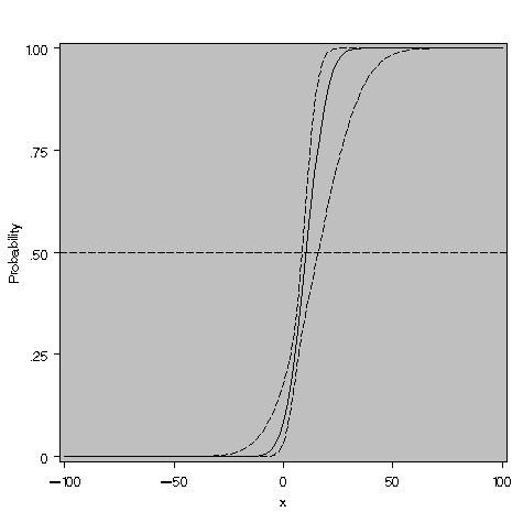
Notice the much tighter confidence bands on the predicted values and that a reference line drawn at a response probability intersects both bands:

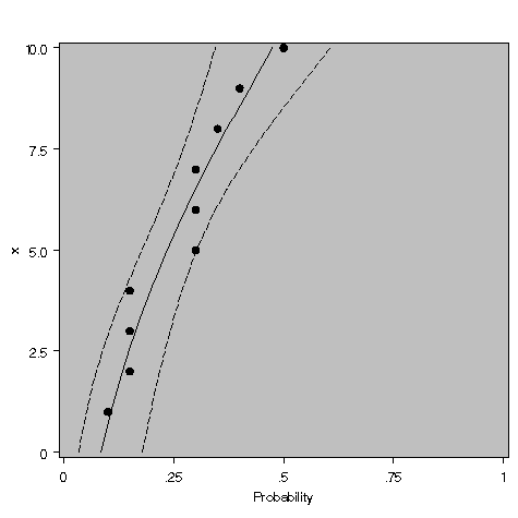
The inverse prediction plot also shows the estimated values and confidence bands:

Operating System and Release Information
| Product Family | Product | System | SAS Release | |
| Reported | Fixed* | |||
| SAS System | SAS/STAT | All | n/a | |
| Type: | Usage Note |
| Priority: | low |
| Topic: | SAS Reference ==> Procedures ==> PROBIT Analytics ==> Categorical Data Analysis Analytics ==> Regression |
| Date Modified: | 2003-04-18 08:24:21 |
| Date Created: | 2002-12-16 10:56:40 |