Usage Note 22571: Comparing the proportions of positive response in several groups to the overall proportion
A single test of whether any of the group proportions differs from the overall proportion is given by the CHISQ option in PROC FREQ when applied to a G×2 or 2×G table of your data (the two columns or rows being positive and negative response). Significant results indicate that at least one proportion differs from the overall proportion. Tests and a graph of each group comparison to overall can be done in PROC LOGISTIC using the DIFF=ANOM option in the LSMEANS statement. You can also adjust the individual p-values for multiple testing. In addition to the adjustments available using the ADJUST= option in the LSMEANS statement in LOGISTIC, the p-values can also be adjusted by importing them into PROC MULTTEST and using the methods available in that procedure.
The sample sizes (N) and the number that respond positive (Npos) in each of five groups are recorded in a SAS data set named P. The observed proportion (Npos/N) is also computed.
| 6 |
46 |
0.13043 |
| 9 |
49 |
0.18367 |
| 9 |
52 |
0.17308 |
| 12 |
54 |
0.22222 |
| 17 |
46 |
0.36957 |
|
These statements transform the above summarized data into the form suitable to produce a 2×2 table for analysis in PROC FREQ. The CHISQ option produces a test of whether the groups all have equal positive response (Response=1) probabilities.
      data p2;
         set p;
         Response=1; Count=Npos; output;
         Response=0; Count=N-Npos; output;
         run;
      proc freq data=p2;
        weight Count;
        table Group*Response / chisq;
        run;
The marginally significant Pearson chi-square test from PROC FREQ indicates that some proportions might differ from the overall proportion (p=0.0537). The Likelihood Ratio chi-square (equivalent in large samples) provides a similar result.
| 4 |
9.3167 |
0.0537 |
| 4 |
8.7694 |
0.0671 |
| 1 |
7.1847 |
0.0074 |
| |
0.1942 |
|
| |
0.1907 |
|
| |
0.1942 |
|
|
The following statements fit a one-way logistic model. The LSMEANS statement estimates the group log odds and proportions. Note that the GLM parameterization (PARAM=GLM) of the GROUP levels must be used in order to use the LSMEANS statement. The ILINK option provides the group probability estimates (labeled "Mean"). The DIFF=ANOM option compares the five group proportions to the overall proportion. The ADJUST=BON option adjusts the p-values using the Bonferroni method. The ODS OUTPUT statement saves the comparisons table to a data set for later use as described below. Note that if there are covariates in addition to your Group variable, they can be added to the model and the LSMEANS statement will provide the comparisons adjusted for the effects of the covariates.
      proc logistic data=p;
         class Group / param=glm;
         model Npos/N = Group;
         lsmeans Group / ilink diff=anom adjust=bon;
         ods output Diffs=GrpDiffs;
         run;
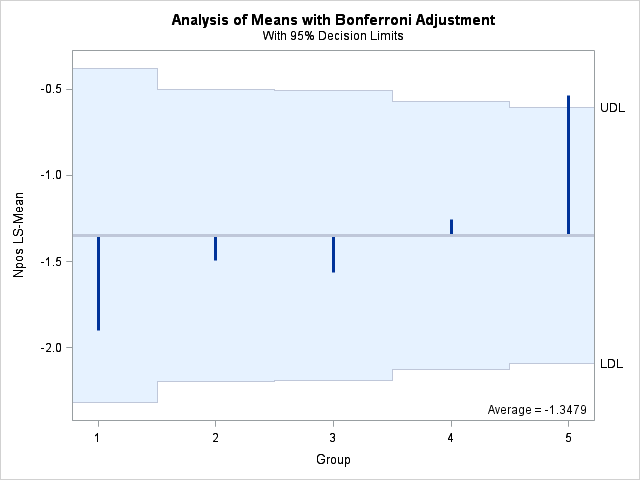
Note that the likelihood ratio chi-square test from PROC FREQ matches the one in the "Testing Global Null Hypothesis: BETA=0" table from PROC LOGISTIC. The "Group Least Squares Means" table provides the group log odds (Estimate column) and proportions (Mean column). The results shown in the "Differences of Group Least Squares Means" table indicate that only the last group differs from overall (raw p=0.0046, Bonferroni-adjusted p=0.0230). The LSMEANS statement provides a plot comparing each group's log odds with the overall log odds (-1.3479). If a group's bar extends beyond the Bonferroni-adjusted upper or lower decision limit (UDL or LDL), then that group's log odds and proportion differ significantly from overall. By default, the significance level for the decision limits is 0.05. The plot visually confirms the conclusion from PROC LOGISTIC that only the last group differs from overall.
| 8.7694 |
4 |
0.0671 |
| 9.3167 |
4 |
0.0537 |
| 8.8401 |
4 |
0.0652 |
| 1 |
-1.8971 |
0.4378 |
-4.33 |
<.0001 |
0.1304 |
0.04966 |
| 2 |
-1.4917 |
0.3689 |
-4.04 |
<.0001 |
0.1837 |
0.05532 |
| 3 |
-1.5640 |
0.3666 |
-4.27 |
<.0001 |
0.1731 |
0.05246 |
| 4 |
-1.2528 |
0.3273 |
-3.83 |
0.0001 |
0.2222 |
0.05658 |
| 5 |
-0.5341 |
0.3055 |
-1.75 |
0.0804 |
0.3696 |
0.07117 |
| 1 |
Avg |
-0.5492 |
0.3762 |
-1.46 |
0.1443 |
0.7215 |
| 2 |
Avg |
-0.1437 |
0.3289 |
-0.44 |
0.6621 |
1.0000 |
| 3 |
Avg |
-0.2161 |
0.3273 |
-0.66 |
0.5092 |
1.0000 |
| 4 |
Avg |
0.09516 |
0.3013 |
0.32 |
0.7522 |
1.0000 |
| 5 |
Avg |
0.8138 |
0.2872 |
2.83 |
0.0046 |
0.0230 |
|
If desired, any of the p-value adjustment methods available in PROC MULTTEST (except the resampling-based bootstrap or permutation methods) can be used to adjust the difference p-values. The ODS OUTPUT statement above saved the p-values to a data set named GrpDiffs. In that data set, the variable containing the raw p-values is named Probz. Use the INPVALUES(variable-name)=data-set-name option in PROC MULTTEST to read the set of p-values. Specify the appropriate option for your choice of nonresampling-based adjustment method. Below, the BON option is used to again to provide the Bonferroni adjustment. The HOLM option is also used to provide the more powerful stepdown Bonferroni adjustment.
      proc multtest inpvalues(Probz)=GrpDiffs bon holm;
         run;
The results show that the adjusted p-values from the stepdown method are very similar to the ordinary Bonferroni method in this case.
| 1 |
0.1443 |
0.7215 |
0.5772 |
| 2 |
0.6621 |
1.0000 |
1.0000 |
| 3 |
0.5092 |
1.0000 |
1.0000 |
| 4 |
0.7522 |
1.0000 |
1.0000 |
| 5 |
0.0046 |
0.0230 |
0.0230 |
|
Operating System and Release Information
*
For software releases that are not yet generally available, the Fixed
Release is the software release in which the problem is planned to be
fixed.
| Type: | Usage Note |
| Priority: | low |
| Topic: | Analytics ==> Analysis of Means
SAS Reference ==> Procedures ==> FREQ
SAS Reference ==> Procedures ==> MULTTEST
Analytics ==> Categorical Data Analysis
Analytics ==> Descriptive Statistics
SAS Reference ==> Procedures ==> LOGISTIC
|
| Date Modified: | 2006-05-10 11:19:08 |
| Date Created: | 2002-12-16 10:56:38 |