Modeling and Forecasting Task
About the Modeling and Forecasting Task
The Modeling and Forecasting task creates forecasting models that use your time series data. This task requires data in a valid time series format. To create this data, use the Time Series Data Preparation task before running the
Modeling and Forecasting task.

Assigning Data to Roles
To run the Modeling
and Forecasting task, you must assign a column to the Dependent
variable role, and you must specify a forecasting model
type on the Model tab.
|
Roles and Options
|
Description
|
|---|---|
|
Roles
|
|
|
Dependent
variable
|
specifies the dependent variable.
|
|
Additional Roles
|
|
|
Time ID
|
specifies the column
that contains the time ID values.
|
|
Properties
|
|
|
Interval
|
shows the interval for
the time ID variable. For
more information about SAS time intervals, see Understanding SAS Time Intervals.
Note: This value is determined
by the input data set. You cannot change this value in the Modeling
and Forecasting task.
|
|
Multiplier
|
shows the multiplier for the time interval. By default, the multiplier is 1.
Note: This value is determined
by the input data set. You cannot change this value in the Modeling
and Forecasting task.
|
|
Shift
|
shows the shift for
the time interval. By default, the shift is 1.
Note: This value is determined
by the input data set. You cannot change this value in the Modeling
and Forecasting task.
|
|
Season length
|
specifies the seasonality of the time interval. The default value depends on the time interval.
|
|
Additional Roles
|
|
|
Season length
|
enables you to specify
the seasonality of the data when you do not assign a time ID variable.
|
|
Group analysis
by
|
lists the variable or
variables that you want to use as the classification (BY) variables.
|
Setting the Model Options
To use the Modeling and Forecasting task, you must
select a forecasting model type. You can choose from six model types:
random walk, moving average, exponential smoothing, ARIMA, ARIMAX,
and unobserved components.
Random Walk
To create a random
walk model:
-
Select one of these types of random walk models:
-
Drift creates a Random Walk model with Drift, or in ARIMA notation ARIMA(0, 1, 0).
-
Trend .
-
Seasonal creates a Seasonal Random Walk model, or ARIMA(0, 1, 0)(0, 1, 0)s with no intercept.
-
-
Under the Plots heading, select the plots to include in the results. You can choose from a variety of series plots, residual plots, and forecast plots.
Moving Average
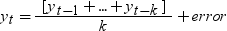
In ARIMA notation, this model is ARIMA(k, 0, 0) with no intercept and with the autoregressive parameters (AR) fixed: 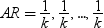 .
.
.
To create a moving
average model:
-
In the Window (periods) box, specify the number of periods for the moving average. This value must be an integer greater than 0 and less than 14.
-
Under the Plots heading, select the plots to include in the results. You can choose from a variety of series plots, residual plots, and forecast plots.
Exponential Smoothing
Exponential smoothing is a forecasting technique that uses exponentially declining weights to produce a weighted moving
average of time series values. You can choose from several forecasting models.
To create an exponential
smoothing model:
-
From the Forecasting model drop-down list, select the model that you want to use. You can choose from these models.
-
Simple (single) exponential smoothing, which is the default
-
Double (Brown) exponential smoothing
-
Linear (Holt) exponential smoothing
-
Damped trend exponential smoothing
-
Additive seasonal exponential smoothing
-
Multiplicative seasonal exponential smoothing
-
Winters multiplicative model
-
Winter additive model
-
-
From the Transformation drop-down list, select the transformation to apply to the time series. By default, no transformation is applied. If you select the Box-Cox transformation, then you must specify a parameter value between -5 and 5 in the Box-Cox transformation parameter box.
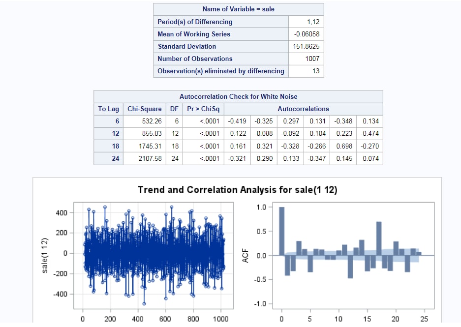
ARIMA
When you create an Autoregressive Integrated Moving Average (ARIMA) model, you can
specify the autoregressive and moving average polynomials of an ARIMA model.
To create an ARIMA
model:
-
Under the ARIMA heading, specify the autoregressive, differencing, and moving average orders for the ARIMA model.Here are the options for the simple ARIMA:
-
Autoregressive order (p) specifies the simple autoregressive order. You can specify an integer from 0 to 13. The default value is 0.
-
Differencing order (d) specifies the simple differencing order. You can specify an integer from 0 to 13. The default value is 0.
-
Moving average order (q) specifies the simple moving average. You can specify an integer from 0 to 13. The default value is 0.
Here are the options for the seasonal ARIMA:-
Autoregressive order (P) specifies the seasonal autoregressive order. You can specify an integer from 0 to 5. The default value is 0.
-
Differencing order (D) specifies the simple differencing order. You can specify an integer from 0 to 3. The default value is 0.
-
Moving average order (Q) specifies the simple moving average. You can specify an integer from 0 to 5. The default value is 0.
-
-
Specify whether to include the intercept in the model. The intercept is included by default.
ARIMAX
When you create an Autoregressive Integrated Moving Average (ARIMA) model, you can
specify the autoregressive and moving average polynomials of an ARIMA model. In an
ARIMAX model, you can also include independent variables in the model.
To create an ARIMAX
model:
-
Under the ARIMA heading, specify the autoregressive, differencing, and moving average orders for the ARIMA model.Here are the options for the simple ARIMA:
-
Autoregressive order (p) specifies the simple autoregressive order. You can specify an integer from 0 to 13. The default value is 0.
-
Differencing order (d) specifies the simple differencing order. You can specify an integer from 0 to 13. The default value is 0.
-
Moving average order (q) specifies the simple moving average. You can specify an integer from 0 to 13. The default value is 0.
Here are the options for the seasonal ARIMA:-
Autoregressive order (P) specifies the seasonal autoregressive order. You can specify an integer from 0 to 5. The default value is 0.
-
Differencing order (D) specifies the simple differencing order. You can specify an integer from 0 to 3. The default value is 0.
-
Moving average order (Q) specifies the simple moving average. You can specify an integer from 0 to 5. The default value is 0.
-
-
In the Independent variables role, assign the variables from the input data set that you want to include in the model.
Unobserved Components
To create an unobserved
components model:
-
To include an irregular component, expand the Irregular Component heading and select the Include an irregular component check box. An irregular component is included by default.The irregular component corresponds to the overall random error in the model. The initial variance is the value used as the initial value during the parameter estimation process. To change this value, select Specify variance and enter a different value. To keep this value as your initial variance, select Fix variance value.
-
To include a trend component, expand the Trend Component heading. The level component and the slope component combine to define the trend component for the model. If you specify both a level and slope component, then a locally linear trend is obtained. If you omit the slope component, then a local level is used.
-
(Optional) To include a seasonal component, the season length must be greater than one. Expand the Seasonal Component heading and select the Include a seasonal component check box. Specify the type of seasonal component. A seasonal component can be one of two types: dummy or trigonometric. You can also specify whether to change the initial variance (which is 0 by default).
-
(Optional) To include a cycle component, expand the Cycle Component heading and select the Include a cycle component check box. You can specify these options:
-
To specify an initial cycle period to use during the parameter estimation process, select the Specify cycle period check box. Then specify the initial value in the box. This value must be an integer greater than 2. By default, the initial value is 3.
-
To specify an initial damping factor to use during the parameter estimation process, select the Specify damping factor check box, and then specify the initial value in the box. You can specify any value between 0 and 1 (excluding 0 but including 1). By default, the initial value is 0.01.
-
To specify an initial value for the disturbance variance parameter that the task uses during the parameter estimation process, select the Specify variance check box. Then specify the initial value in the box. This value must be greater than or equal to 0. By default, the initial value is 0.
-
-
Under the Plots heading, select the plots to include in the results. You can choose from a variety of residual plots, smoothed component estimates, filtered component estimates, and series decomposition and forecast plots.
Setting the Forecasting Options
|
Option
|
Description
|
|---|---|
|
Forecast Settings
|
|
|
Number of
periods to forecast
|
specifies the number of periods into the future for which multistep forecasts are made. The larger the horizon value, the larger the prediction error variance at the end of the horizon. By default, the horizon is 12. Valid values are
integers greater than or equal to 0 and less than 32,768.
|
|
Forecast
confidence level
|
specifies the confidence level for the series. By default, this confidence level is 95% .
|
|
Number of
periods to hold back
|
specifies a subset of actual time series values to hold back, starting from the end of the last nonmissing observation. Valid values are integers greater than or equal to 0 and less than 32,768.
|
|
Outlier Detection
Note: This option is not available
if you selected Exponential smoothing as
the forecasting model type.
|
|
|
Perform
outlier detection
|
specifies that any outliers that are automatically detected during the creation of the model are inputs in the
model.
|
Setting the Output Options
To create an output data set, click the Output tab. The types of output data sets that you can create depend on the forecasting model type.
Copyright © SAS Institute Inc. All rights reserved.