Time Series Data Preparation Task :: SAS(R) Studio 3.4: User's Guide

About the Time Series Data Preparation Task

The Time Series Data Preparation task turns time-stamped transactional data into equally spaced time series data. This format is required for further time series analysis. This task does not require a time ID variable. If no time ID variable is specified, the observation number is the ID for the time series.

Understanding SAS Time Intervals

The Time Data Preparation task analyzes the variable assigned to the time ID role to detect the time interval of the data. SAS assumes that all the values in the time ID variable are either date or datetime values and distinguishes between the values by their magnitude. This assumption fails if you have dates that extend beyond July 21, 2196, or datetimes before January 1, 1960.

For many businesses, their time series data is equally spaced, or any two consecutive indices have the same difference between the time intervals. The following table shows an equally spaced time series with a one-year interval.

Year	Number of Sales
2012	42,100
2013	45,000
2014	47,000
2015	50,000

If the time interval cannot be detected from the variable that you assign, then you need to specify the interval and season length. For example, the following table shows an unequally spaced time series.

Year	Number of Sales
2009	32,100
2010	45,000
2014	47,000
2015	50,000

Often the time interval cannot be detected with transactional data (time-stamped data that is recorded at no particular frequency). If this is the case, the task accumulates the data into observations that correspond to the interval that you specify. For nontransactional data, you might need to specify the interval and season length if there are numerous gaps (missing values) in the data. In this case, the task supplies the missing values. A validation routine checks the values of the time ID to determine whether they are spaced according to the interval that you specified.

The interval determines the frequency of the output. You can modify the time interval. You can change the interval from a higher frequency to a lower frequency or from a lower frequency to a higher frequency. Time intervals are specified in SAS by using character strings. Each of these strings is formed according to a set of rules that enables you to create an almost infinite set of attributes. For each time interval, you can specify the type (such as monthly or weekly), a multiplier, and a shift (the offset for the interval). You can specify a greater time interval than that found in the input data. A smaller interval should not be used, because a small interval generates a large number of observations.

Seasonal cycle length specifies the length of a season. This value is populated automatically if the task can determine the season length from the time ID variable. However, you can specify a season length other than the default if you want to model a cycle in the data. For example, your data might contain a 13-week cycle, so you need to specify a 13-week season length.

Here is the syntax for an interval:

name<multipler><.shift>

Here is an explanation of each of the user-supplied values:

name

is the name of the interval.

multipler

specifies the multiplier of the interval. This value can be any positive number. By default, the multiplier is 1. For example, YEAR2 indicates a two-year interval.

.shift

specifies the starting point for the interval. By default, this value is one. A value greater than 1 shifts the start to a later point within the interval. The unit for the shift depends on the interval. For example, YEAR.4 specifies a shift of four months, so the year is from April 1 through March 31 of the following year.

The examples in the following table show how the values that you specify for the interval, season length, multiplier, and shift work together.

Interval Name (in SAS Code Format)	Default	Shift Period	Example
YEARm.s	January 1	Months	YEAR2.7 specifies an interval of every two years. Because the value for the shift is 7, the first month in the year is July.
QTRm.s	January 1 April 1 July 1 October 1	Months	QTR3.2 specifies three-month intervals starting on April 1, July 1, October 1, and January 1.
MONTHm.s	First of each month	Months	MONTH2.2 specifies February–March, April–May, June–July, August–September, October–November, and December–January of the following year.
WEEKm.s	Each Sunday	Days (1=Sunday . . . 7=Saturday)	WEEK6.3 specifies six-week intervals starting on Tuesdays.
DAYm.s	Each day	Days	DAY3 specifies three-day intervals starting on Sunday.

Example: Transforming the Data in the SASHELP.PRICEDATA Data Set

To create this example:

In the Tasks section, expand the Forecasting folder and double-click Time Series Data Preparation. The user interface for the Time Series Data Preparation task opens.
On the Data tab, select the SASHELP.PRICEDATA data set.

Assign columns to these roles:

Role	Column
Roles
Time series variable	sale price1
Additional Roles
Time ID	date
Properties
Interval	Quarter

Click the Transformation tab and specify these values for the sale variable.
- From the Accumulation drop-down list, select Sum.
- From the Transformation drop-down list, select Logarithmic.
- In the Simple Difference box, enter 1.
- In the Seasonal Difference box, enter 0.
For the price variable, select Sum from the Accumulation drop-down list.
Click the Output tab. Select the Show output data check box. In the Number of observations to show box, enter 10.
To run the task, click .

Here are the results:

Assigning Data to Roles

To run the Time Series Data Preparation task, you must assign a column to the Time series variable role.

Role	Description
Roles
Time series variable	lists the variables that contain time-stamped data
Treatment of missing values	specifies how to treat missing values in the time-stamped data. You can choose from these options: Missing value Average value of the accumulated time series Minimum value of the accumulated time series Median value of the accumulated time series Maximum value of the accumulated time series First nonmissing value of the accumulated time series Last nonmissing value of the accumulated time series The previous period’s accumulated nonmissing value The missing values are set to the previous accumulated nonmissing value. Missing values at the beginning of the accumulated series remain missing. The next period’s accumulated nonmissing value The missing values are set to the next accumulated nonmissing value. Missing values at the end of the accumulated series remain missing. Numeric value specifies the value to use for the missing value.
Additional Roles
Time ID	specifies the column that contains the time ID values.
Properties
Interval	specifies the interval for the time ID variable. For more information about time intervals, see Understanding SAS Time Intervals.
Multiplier	specifies the multiplier for the time interval. By default, the multiplier is 1. This value cannot be negative.
Shift	specifies the shift for the time interval. By default, the shift is 1. This value cannot be negative.
Season length	specifies the seasonality of the time interval. The default value depends on the time interval.
Additional Roles
Season length	enables you to specify the seasonality of the data when you do not assign a time ID variable.
Group analysis by	lists the variable or variables that you want to use as the classification (BY) variables.

Setting the Transformations Options

The Transformations table contains a row for each column that you assigned to the Time series variable role.

Option Name	Description
Accumulation	specifies the accumulation method for the variable. This option is available if you assigned a variable to the Time ID variable role. You can choose from these options: None does not accumulate the vector values. Sum accumulates the vector values based on the summation of their values. Missing values are ignored in the summation. If , then a is set to missing. Average accumulates the vector values based on the average of their values. $eh equals , r with macron above , equals , fraction 1 , over q sub n end fraction . cap sigma with q equals 1 below and with q above . r sub q. Click image for alternative formats.$ Missing values are ignored in the summation. If , then a is set to missing.
Transformation	specifies the transformation to apply to the time series variable. You can choose from these transformations: Logarithmic Square-root Logistic
Simple differencing	specifies a value for the simple difference.
Seasonal differencing	specifies a value for the seasonal difference. This option is available if the value of the Seasonal length option on the Data tab is greater than 1.

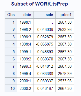
Creating the Output Data Set

The Show output data check box specifies whether to include the output data in the results that appear on the Results tab. You can include all or a subset of the output data. The task always creates the output data set that appears on the Output Data tab. This data set is also saved to the specified location.