Generalized Linear Models :: SAS(R) Studio 3.3: User's Guide

About the Generalized Linear Models Task

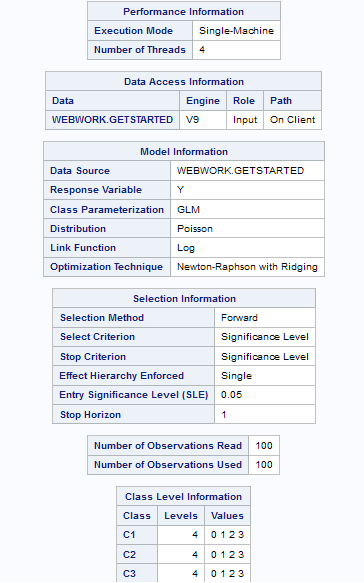
The Generalized Linear Models task is a high-performance task that provides model fitting and model building for generalized linear models. It fits models for standard distributions such as Normal, Poisson, and Tweedie in the exponential family. This task also fits multinomial models for ordinal and nominal responses. The task provides forward, backward, and stepwise selection methods.

Note: This task is available only if you are running SAS 9.4 or later.

Example: Model Selection

To create this example:

Create the Work.getStarted data set. For more information, see GETSTARTED Data Set.
In the Tasks section, expand the High-Performance Statistics folder and double-click Generalized Linear Models. The user interface for the Generalized Linear Models task opens.
On the Data tab, select the WORK.GETSTARTED data set.

Assign columns to these roles:

Role or Option Name	Column Name
Distribution	Poisson
Response variable	Y
Classification variables	C1 C2 C3 C4 C5

Click the Model tab. In the Variables box, select C1–C5. Click Add.
Click the Selection tab. From the Selection method drop-down list, select Forward selection.
To run the task, click .

Here is a subset of the results:

Performance Information, Model Information, Selection Information, and Class Level Information

Assigning Data to Roles

To run the Generalized Linear Models task, you must assign a column to the Response variable role.

Option Name	Description
Roles
Response
Distribution	specifies the distribution for your model. You can choose from these distributions: Binomial Gamma Inverse Gaussian Multinomial Negative binomial Normal Poisson Tweedie
Options for Binomial Distribution
Response data consists of numbers of events and trials	specifies whether the data consists of a variable that specifies the number of positive responses (events) and another variable that specifies the number of trials.
Number of events	specifies the column that contains the number of events.
Number of trials	specifies the column that contains the number of trials.
Response	specifies the variable that contains response values. If you create a binomial response model, you can specify the first or last ordered category as the reference category by using the Event of interest option. You can also select a custom category. Note: This option is available only if you do not select the Response data consists of numbers of events and trials check box.
Options for All Distribution Types
Response	specifies the variable that contains response values. If you create a binomial response model or a nominal multinomial model, you can specify the first or last ordered category as the reference category by using the Event of interest option. You can also select a custom category. To create a binomial response model, select Binomial as the distribution. For the binomial response model, specifying one response category as the reference is the same as specifying the other response category as the event category. To create a nominal multinomial model, select Multinomial as the distribution and select Generalized logit as the link function. For the generalized logit model, each logit contrasts a nonreference category with the reference category.
Link function	specifies the link function for your model. The functions that are available depend on the selected distribution. If you select Default for the link function, then the default link function for the model distribution is used. Here is the list of distributions with the corresponding default link function: Binomial distribution uses the logit link function. Gamma distribution uses the reciprocal link function. Inverse Gaussian distribution uses the reciprocal square link function. Multinomial distribution uses the cumulative logit link function. Negative binomial distribution uses the log link function. Normal distribution uses the identity link function. Poisson distribution uses the log link function. Tweedie distribution uses the log link function.
Explanatory Variables
Classification variables	specifies the variables to use to group (classify) data in the analysis. Classification variables can be either character or numeric.
Parameterization of Effects
Coding	specifies the parameterization method for the classification variable. Design matrix columns are created from the classification variables according to the selected coding scheme. You can select from these coding schemes: GLM coding specifies less-than-full-rank, reference-cell coding. This coding scheme is the default. Reference coding specifies reference-cell coding.
Treatment of Missing Values
An observation is excluded from the analysis when either of these conditions is met: if any variable in the model contains a missing value if any classification variable contains a missing value (regardless of whether the classification variable is used in the model)
Continuous variables	specifies the independent covariates (regressors) for the regression model. If you do not specify a continuous variable, the task fits a model that contains only an intercept.
Offset variable	specifies a variable to be used as an offset to the linear predictor. An offset plays the role of an effect whose coefficient is known to be 1. Observations that have missing values for the offset variable are excluded from the analysis.
Additional Roles
Frequency count	specifies the numeric column that contains the frequency of occurrence for each observation.
Weight variable	specifies the column to use as a weight to perform a weighted analysis of the data.

Building a Model

Requirements for Building a Model

By default, no effects are specified, which results in the task fitting an intercept-only model. To specify an effect, you must assign at least one variable to the Classification variables role or the Continuous variables role. You can select combinations of variables to create crossed, nested, factorial, or polynomial effects.

To create a model, use the model builder on the Models tab. After you create a model, you can specify whether to include the intercept in the model.

Create a Main Effect

Select the variable name in the Variables box.
Click Add to add the variable to the Model effects box.

Create Crossed Effects (Interactions)

Select two or more variables in the Variables box. To select more than one variable, press Ctrl.
Click Cross.

Create a Nested Effect

Nested effects are specified by following a main effect or crossed effect with a classification variable or list of classification variables enclosed in parentheses. The main effect or crossed effect is nested within the effects listed in parentheses. Here are examples of nested effects: B(A), C(B*A), D*E(C*B*A). In this example, B(A) is read "A nested within B."

Select the effect name in the Model effects box.
Click Nest. The Nested window opens.
Select the variable to use in the nested effect. Click Outer or Nested within Outer to specify how to create the nested effect.

Note: The Nested within Outer button is available only when a classification variable is selected.
Click Add.

Create a Full Factorial Model

Select two or more variables in the Variables box.
Click Full Factorial.

For example, if you select the Height, Weight, and Age variables and then click Full Factorial, these model effects are created: Age, Height, Weight, Age*Height, Age*Weight, Height*Weight, and Age*Height*Weight.

Create an N-Way Factorial

Select two or more variables in the Variables box.
Click N-way Factorial to add these effects to the Model effects box.

For example, if you select the Height, Weight, and Age variables and then specify the value of N as 2, when you click N-way Factorial, these model effects are created: Age, Height, Weight, Age*Height, Age*Weight, and Height*Weight. If N is set to a value greater than the number of variables in the model, N is effectively set to the number of variables.

Create Polynomial Effects of the Nth Order

Select one variable in the Variables box.
Specify higher-degree crossings by adjusting the number in the N field.
Click Polynomial Order=N to add the polynomial effects to the Model effects box.

For example, if you select the Age and Height variables and then you specify 3 in the N field, when you click Polynomial Order=N, these model effects are created: Age, Age*Age, Age*Age*Age, Height, Height*Height, and Height*Height*Height.

Setting the Model Selection Options

Option	Description
Model Selection
Selection method	specifies the selection method for the model. The task performs model selection by examining whether effects should be added to or removed from the model according to the rules that are defined by the selection method. Here are the valid values for the selection methods: None fits the full model. Forward selection starts with no effects in the model and adds effects based on the Significance level to add an effect to the model option.
Selection method (continued)	Backward elimination starts with all the effects in the model and deletes effects based on the value in the Significance level to remove an effect from the model option. Stepwise selection is similar to the forward selection model. However, effects that are already in the model do not necessarily stay there. Effects are added to the model based on the Significance level to add an effect to the model option and are removed from the model based on the Significance level to remove an effect from the model option.
Select best model by	specifies the criterion to use to identify the best-fitting model.
Details
Selection process details	specifies how much information about the selection process to include in the results. You can display a summary, details for each step of the selection process, or all of the information about the selection process.
Maintain hierarchy of effects	specifies to maintain the hierarchy of effects.

Setting Options

Option	Description
Methods
Dispersion
Dispersion parameter	enables you to specify a fixed dispersion parameter for those distributions that have a dispersion parameter. By default, this parameter is estimated.
Optimization
Method	specifies the optimization technique to use.
Maximum number of iterations	specifies the maximum number of iterations to perform for the selected optimization technique.
Statistics
You can select the statistics to include in the output. Here are the additional statistics that you can include: confidence limits for estimates correlations of parameter estimates covariances of parameter estimates

Setting the Output Options

You can specify whether to create an output data set. You can also specify whether to include predicted values, residuals, or any other variables in the output data set.