Data Exploration Task

About the Data Exploration Task

Example: Exploring the SASHELP.CARS Data

Assigning Data to Roles

Setting the Plot Options

About the Data Exploration Task

The Data Exploration task provides graphs that can be used to explore the relationships among selected variables.

Example: Exploring the SASHELP.CARS Data

To create this example:

In the Tasks section, expand the Statistics folder and double-click Data Exploration. The user interface for the Data Exploration task opens.
On the Data tab, select the SASHELP.CARS data set.

Assign columns to these roles and specify these options:

Role	Column Name
Continuous variables	Horsepower MPG_City MPG_Highway
Classification variables	Type DriveTrain

To run the task, click .

Here is a subset of the results:

Scatter Plot Matrix of Sashelp.Cars Data Grouped by Type

Scatter Plot Matrix of Sashelp.Cars Grouped by DriveTrain

Assigning Data to Roles

To run the Data Exploration task, you must assign either two columns to the Classification variables role or one column to the Continuous variables role.

Role	Description
Roles
Classification variables	specifies the classification variables to use to explore the data.
Continuous variables	specifies the continuous variables in the analysis.
Additional Roles
Group analysis by	creates separate analyses based on the number of BY variables.

Setting the Plot Options

The plot options that are available depend on the columns that you assigned on the Data tab.

Option Name	Description
Histogram and Box Plot
The combined histogram and box plot options are available when a column is assigned to the Continuous variables role, but no column is assigned to the Classification variables role.
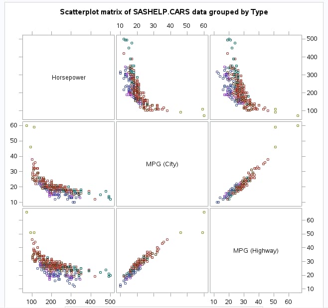
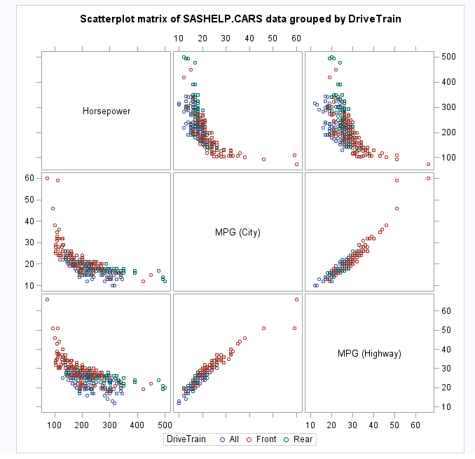
Scatter Plot Matrix
The scatter plot matrix options are available when at least two columns are assigned to the Continuous variables role.
Add histograms	adds histograms to the diagonal cells of the matrix. You can add a normal density curve and the kernel density estimate to these histograms.
Add prediction ellipses	adds a prediction ellipse to each cell that contains a scatter plot. You can specify the confidence level for the ellipses. Valid values are between 0 and 1.
Pairwise Scatter Plots
The pairwise scatter plot options are available when at least two columns are assigned to the Continuous variables role.
Pairwise scatter plots	plots the values of two or more variables and produces a separate cell for each combination of Y and X variables. That is, each Y*X pair is plotted on a separate set of axes.
Add a prediction ellipse	adds a prediction ellipse to each cell that contains a scatter plot. You can specify the confidence level for the ellipses. Valid values are between 0 and 1.
Regression Scatter Plots
The regression scatter plot options are available when at least two columns are assigned to the Continuous variables role.
Regression scatter plots	adds a regression fit to the scatter plot.
Select response variables	specifies the variables to use when fitting the regression line.
Add a fitted line	adds a regression fit to the scatter plot.
Add a loess fit	adds a loess fit to the scatter plot.
Add a fitted, penalized B-spline curve	adds a fitted, penalized B-spline curve to the scatter plot.
Mosaic Plot
Mosaic plot	creates a mosaic plot, which displays tiles that correspond to the crosstabulation table cells. The areas of the tiles are proportional to the frequencies of the table cells. The column variable is displayed on the X axis, and the tile widths are proportional to the relative frequencies of the column variable levels. The row variable is displayed on the Y axis, and the tile heights are proportional to the relative frequencies of the row levels within column levels.
Square mosaic plot	produces a square mosaic plot, where the height of the Y axis equals the width of the X axis. In a square mosaic plot, the scale of the relative frequencies is the same on both axes.
Specify colors of mosaic plot tiles	colors the mosaic plot tiles according to the values of residuals. You can also specify to color the tiles according to the Pearson or standardized residuals of the corresponding table cells.
Histogram
Histogram	creates a histogram by using any numeric variables in the input data set.
Add normal density curve	adds a normal density curve to the histogram.
Add kernel density estimate	adds a kernel density estimate to the histogram.
Add inset statistics	adds a box or table of summary statistics directly in the histogram.
Box Plot
The box plot options are available when at least one column is assigned to the Classification variables role.
Comparative box plot	creates a one-way box plot for each classification variable. This plot shows all continuous variables by the classification variable.