Nonparametric One-Way ANOVA Task
Assigning Data to Roles
To run the Nonparametric
One-Way ANOVA task, you must assign columns to the Dependent
variable and Classification variable roles.
|
Role Name
|
Description
|
|---|---|
|
Roles
|
|
|
Dependent
variable
|
specifies the column
to use as the dependent variable.
|
|
Classification
variable
|
defines the subgroups.
Separate analyses are performed for each subgroup. You can specify
whether to treat missing values as a valid level.
|
|
Additional Roles
|
|
|
Frequency
count
|
specifies that each
row in the table is assumed to represent n observations.
In this example, n is the value of the frequency
count for that observation.
|
|
Group analysis
by
|
sorts the table by these
columns. The task performs analyses on each group.
|
Setting Options
|
Option Name
|
Description
|
|---|---|
|
Plots
|
|
|
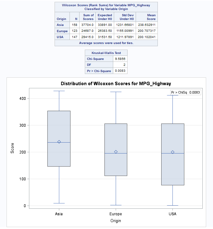
By default, plots are
included in the results. These plots are determined by the options
that you select. Here are some of the plots that you can create:
You can specify whether
to display the p-values in the plot.
To suppress the plots
from the results, select the Suppress plots check
box.
|
|
|
Tests
|
|
|
Tests
|
specifies whether to
calculate only the asymptotic tests or both the asymptotic tests and
exact tests for the various analyses.
|
|
Location Differences
|
|
|
Wilcoxon
scores
|
ranks of the observations.
|
|
Median scores
|
equals 1 for observations
greater than the median and 0 otherwise.
|
|
Van der
Waerden scores
|
the quantiles of a standard
normal distribution. These scores are also known as quantile normal
scores.
|
|
Savage scores
|
the expected values
of order statistics from the exponential distribution with 1 subtracted
to center the scores around 0.
|
|
Scale Differences
|
|
|
Ansari-Bradley
scores
|
similar to the Siegel-Tukey
scores, but assigns the same scores to corresponding extreme ranks.
|
|
Klotz scores
|
the squares of the Van
der Waerden (or quantile normal) scores.
|
|
Mood scores
|
the square of the difference
between each rank and the average rank.
|
|
Siegel-Tukey
scores
|
scores are computed
as
 . .
The score values continue
to increase in this pattern toward the middle ranks until all observations
are assigned a score.
|
|
Location and Scale Differences
|
|
|
Conover
scores
|
based on the squared
ranks of the absolution deviations from the sample means.
|
|
Additional Tests
|
|
|
Empirical
distribution function tests, including Kolmogorov-Smirnov and Cramer-von
Mises tests
|
the empirical distribution
function (EDF) statistics.
|
|
Pairwise
multiple comparison analysis (asymptotic only)
|
computes the Dwass,
Steel, Critchlow-Fligner (DSCF) multiple comparison analyses.
|
|
Methods
|
|
|
Continuity Correction
|
|
|
Continuity
correction for two sample Wilcoxon and Siegel-Tukey tests
|
uses a continuity correction
for the asymptotic two-sample Wilcoxon and Siegel-Tukey tests by default.
The task incorporates this correction when computing the standardized
test statistic z by subtracting 0.5 from the
numerator
 if it is greater than zero. If the numerator is
less than zero, the task adds 0.5. if it is greater than zero. If the numerator is
less than zero, the task adds 0.5.
|
|
Exact Statistics Computation
|
|
|
Use Monte
Carlo estimation
|
requests the Monte Carlo
estimation of the exact p-values instead of
using the direct exact p-value computation.
You can also specify the level of the confidence limits for the Monte
Carlo p-value estimates.
|
|
Limit computation
time
|
specifies the time limit
for calculating each exact p-value. Calculating
exact p-values can consume a large amount of
time and memory.
|
Copyright © SAS Institute Inc. All rights reserved.

