|
|
|
|
|
By default, plots are
included in the results. These plots are determined by the options
that you select. Here are some of the plots that you can create:
-
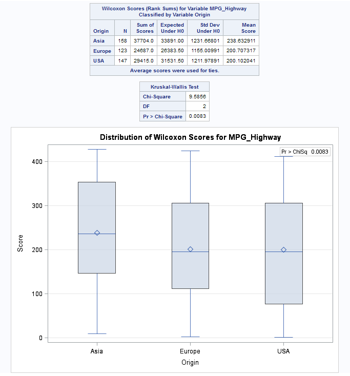
By selecting the options in the Location
Differences section, you can create a box plot of Wilcoxon
scores, a stacked bar chart showing frequencies above or below the
overall median, a box plot of Van der Waerden scores, and a box plot
of Savage scores.
-
By selecting the options in the Scale
Differences section, you can create a box plot of Ansari-Bradley
scores, a box plot of Klotz scores, a box plot of Mood scores, and
a box plot of Siegel-Tukey scores.
-
By selecting the options in the Location
and Scale Differences section, you can create a box plot
of Conover scores.
-
By selecting the Empirical
distribution function tests, including Kolmogorov-Smirnov and Cramer-von
Mises tests option, you can create a plot of the empirical
distribution test.
You can specify whether
to display the p-values in the plot.
To suppress the plots
from the results, select the Suppress plots check
box.
|
|
|
|
|
specifies whether to
calculate only the asymptotic tests or both the asymptotic tests and
exact tests for the various analyses.
|
|
|
|
|
ranks of the observations.
|
|
|
equals 1 for observations
greater than the median and 0 otherwise.
|
|
|
the quantiles of a standard
normal distribution. These scores are also known as quantile normal
scores.
|
|
|
the expected values
of order statistics from the exponential distribution with 1 subtracted
to center the scores around 0.
|
|
|
|
|
similar to the Siegel-Tukey
scores, but assigns the same scores to corresponding extreme ranks.
|
|
|
the squares of the Van
der Waerden (or quantile normal) scores.
|
|
|
the square of the difference
between each rank and the average rank.
|
|
|
scores are computed
as  .
The score values continue
to increase in this pattern toward the middle ranks until all observations
are assigned a score.
|
Location and Scale Differences
|
|
|
based on the squared
ranks of the absolution deviations from the sample means.
|
Empirical
distribution function tests, including Kolmogorov-Smirnov and Cramer-von
Mises tests
|
the empirical distribution
function (EDF) statistics.
|
Pairwise
multiple comparison analysis (asymptotic only)
|
computes the Dwass,
Steel, Critchlow-Fligner (DSCF) multiple comparison analyses.
|
|
|
|
|
Continuity
correction for two sample Wilcoxon and Siegel-Tukey tests
|
uses a continuity correction
for the asymptotic two-sample Wilcoxon and Siegel-Tukey tests by default.
The task incorporates this correction when computing the standardized
test statistic z by subtracting 0.5 from the
numerator  if it is greater than zero. If the numerator is
less than zero, the task adds 0.5.
|
Exact Statistics Computation
|
Use Monte
Carlo estimation
|
requests the Monte Carlo
estimation of the exact p-values instead of
using the direct exact p-value computation.
You can also specify the level of the confidence limits for the Monte
Carlo p-value estimates.
|
|
|
specifies the time limit
for calculating each exact p-value. Calculating
exact p-values can consume a large amount of
time and memory.
|
|
|
You can specify whether
to save the statistics to a data set. By default, the data set is
saved to the Work library.
|