Previous Page

|

Next Page

Skewness

Data can be positively or negatively skewed. The transformations commonly used to improve normality compress the right side of the distribution more than the left side. Consequently, they improve the normality of positively skewed distributions.

For example, look at the histogram of the min_pressure variable in the Hurricanes data, shown in Figure 32.25. The data are negatively skewed.

Figure 32.25: A Negatively Skewed Variable

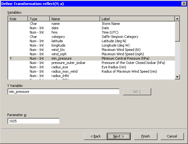
To improve the normality of these data, you first need to reflect the distribution to make it positively skewed. You can reflect data by using the Reflect(Y;a) transformation in the Scaling/Translation family. Reflecting the data about any point accomplishes the goal of reversing the sign of the skewness. The transformation shown in Figure 32.26 uses .

Figure 32.26: Defining a Reflection Transformation

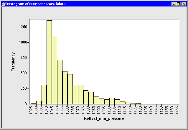
A histogram of the reflected data is shown in Figure 32.27.

Figure 32.27: A Histogram of Reflected Data

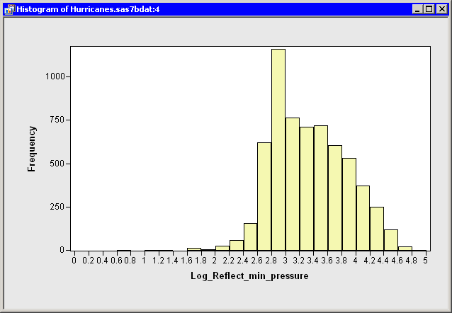
You can now apply a normalizing transformation to the Reflect_min_pressure variable. The minimum value of this variable is 1026. As described in the section "Translating Data", you can translate and apply a logarithmic transformation in a single step: select the log(Y+a) transformation with . A histogram for the logarithmically transformed variable shows improved normality (Figure 32.28), but it is still far from normal.

Figure 32.28: A Histogram of the Logarithm of Reflected Data

Alternatively, you could transform the Reflect_min_pressure variable in two steps: use the a+b*Y transformation with and , and then apply a normalizing transformation. This technique is recommended for transformations (such as the Box-Cox family) that do not have a built-in translation parameter.