Techniques for Exploring Data

Example

In this section, you create many plots of variables in the Hurricanes data set. You use the Workspace Explorer to manage the display of plots.

Open the Hurricanes data set.

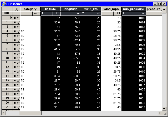
Scroll the data table horizontally until the min_pressure variable appears. Hold down the CTRL key while you select the min_pressure, wind_kts, longitude, and latitude variables, in that order.

Figure 11.16 shows the selected variables. Note that the column headings display numbers that indicate the order in which you selected the variables.

Figure 11.16: Selecting Variables

Select Graph Scatter Plot from the main menu.

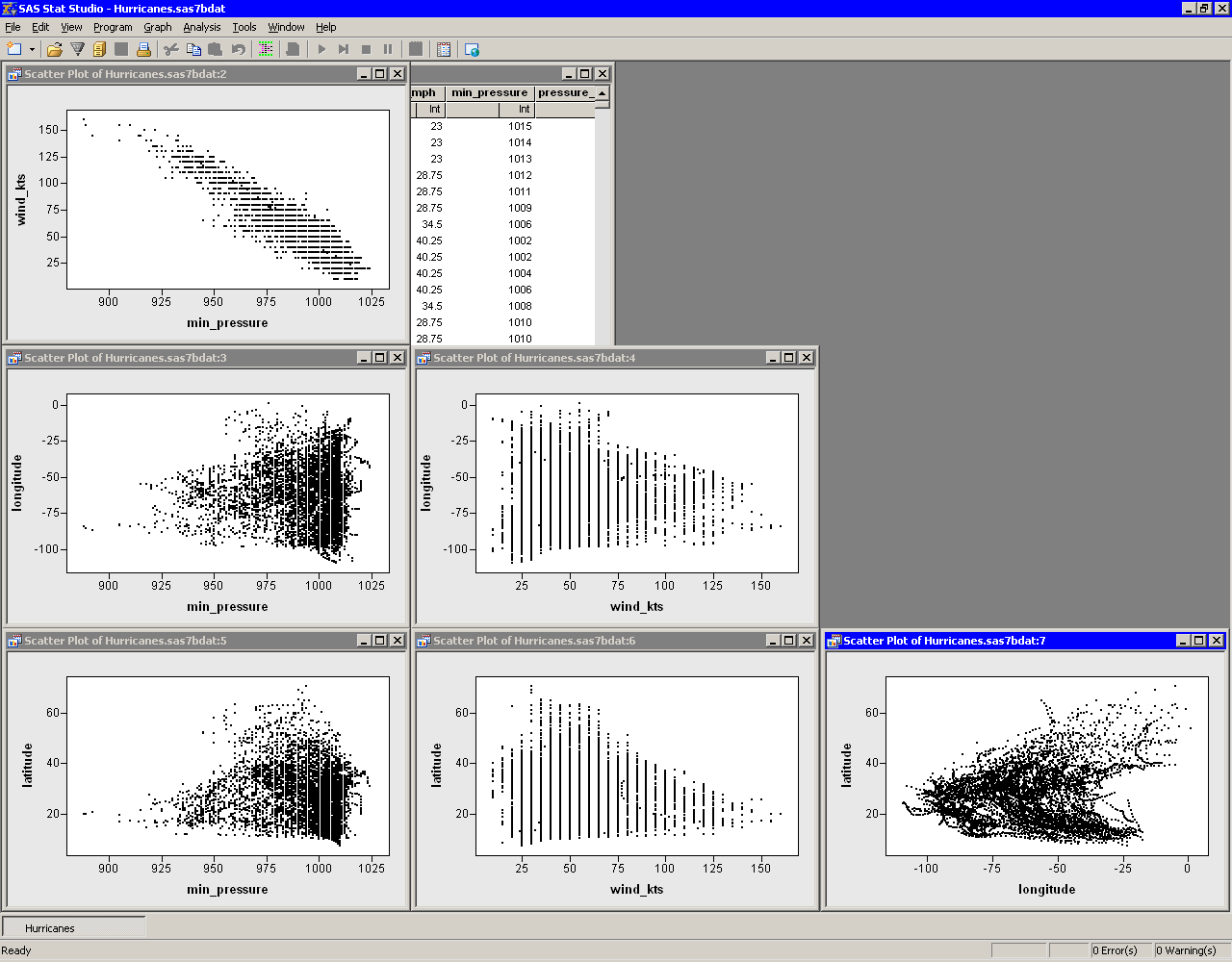
A matrix of scatter plots appears, as shown in Figure 11.17.

Figure 11.17: A Matrix of Scatter Plots

The scatter plot of wind_kts versus min_pressure show a strong negative correlation () between wind speed and pressure. In the following steps, you model the linear relationship between these two variables and create plots of the fit residuals.

Select Analysis Data Smoothing Polynomial Regression from the main menu.

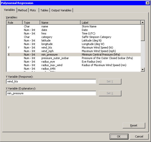
The dialog box shown in Figure 11.18 appears.

Figure 11.18: The Polynomial Regression Dialog Box

Select the variable wind_kts, and click Set Y. Select the variable min_pressure, and click Set X.

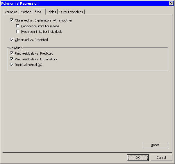
Click the Plots tab, as shown Figure 11.19.

Figure 11.19: The Plots Tab

Select all plots. Clear the check boxes Confidence limits for means and Prediction limits for individuals. Click OK.

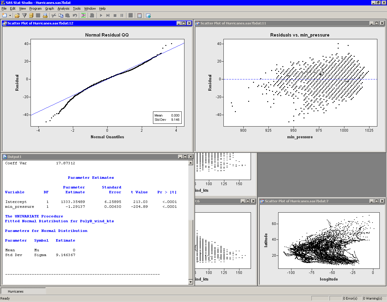
The analysis creates the five requested plots and an output window, as shown in Figure 11.20. Some of the plots produced by the analysis might be hidden beneath other plots.

Figure 11.20: Output and Plots from Polynomial Regression

Your workspace now has a data table, a matrix of six scatter plots, five plots associated with an analysis, and an output window, for a total of 13 windows. The Workspace Explore enables you to manage these windows.

Press ALT+X to open the Workspace Explorer.

The Workspace Explorer is shown in Figure 11.21.

Figure 11.21: The Workspace Explorer

You can use the Workspace Explorer to do the following:

• bring a window or group of windows to the front of other windows
• hide a window or group of windows
• close a window or group of windows

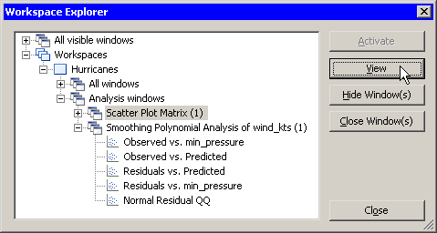
For example, if you want to see all of the windows associated with the scatter plot matrix, you can do the following.

Click on the node labeled Scatter Plot Matrix, and click View.

This step is shown in Figure 11.22. The matrix of scatter plots becomes visible.

Figure 11.22: Viewing a Group of Windows

You also can view a particular plot. For example, the following steps activate the plot containing the least squares line.

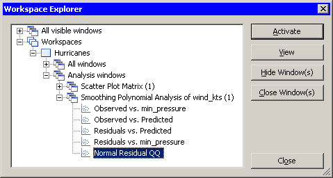
In the Workspace Explorer, expand the node labeled Smoothing Polynomial Analysis of wind_kts, if it is not already expanded.

Click on the item labeled Observed vs. min_pressure.

This step is shown in Figure 11.23. Note that the icon to the left of the plot name indicates that the plot is a scatter plot. The icons in the Workspace Explorer match the icons on the Graph main menu.

Figure 11.23: Activating a Window

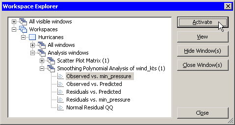
Note that the Activate button is now active, whereas it was previously inactive. This is because the selected item is an individual window instead of a group of windows. Activate behaves similarly to View, but also closes the Workspace Explorer and makes the selected window the active window.

Click Activate.

When you are finished viewing a group of plots, the Workspace Explorer makes it easy to close them. You can close workspaces in the same way.

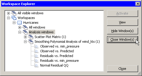
Press ALT+X to open the Workspace Explorer. Click on the node labeled Analysis windows. Click Close Window(s).

This step is shown in Figure 11.24. Stat Studio closes all of the plots created in this example.

Figure 11.24: Closing a Group of Windows

In summary, the Workspace Explorer enables you to view (or hide) windows. The following list describes each button in the Workspace Explorer.

Activate

makes the selected window visible and active. Selecting this button also closes the Workspace Explorer.

View

makes the selected window or group of windows visible.

Hide Window(s)

hides the selected window or group of windows.

Close Window(s)

closes the selected window or group of windows. You can also press the DELETE key to close the selected window or group of windows.

Close

closes the Workspace Explorer.