Multivariate Analysis: Discriminant Analysis

Example

In this example, you examine measurements of 159 fish caught in Finland's Lake Laengelmavesi. The fish are one of seven species: bream, parkki, perch, pike, roach, smelt, and whitefish. Associated with each fish are physical measurements of weight, length, height, and width. The goal of this example is to construct a discriminant function that classifies species based on physical measurements.

Open the Fish data set.

Select Analysis Multivariate Analysis Discriminant Analysis from the main menu, as shown in Figure 30.1.

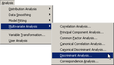
Figure 30.1: Selecting the Discriminant Analysis

A dialog box appears as in Figure 30.2. You can select variables for the analysis by using the Variables tab.

Select Species and click Set Y.

Select Weight. While holding down the CTRL key, select Length1, Length2, Length3, Height, and Width. Click Add X.

Note: Alternately, you can select the variables by using contiguous selection: click on the first variable (Weight), hold down the SHIFT key, and click on the last variable (Width). All variables between the first and last item are selected and can be added by clicking Add X.

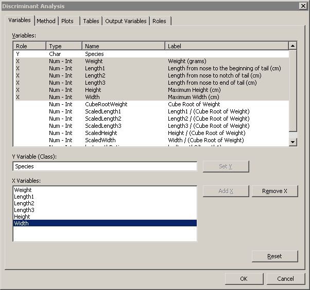
Figure 30.2: The Variables Tab

Click the Method tab.

The Method tab (Figure 30.3) becomes active. You can use the Method tab to set options in the analysis.

Select Kernel density for Classification method.

The options associated with the kernel density classification method become active.

Select Normal for Kernel.

The number of fish in the lake probably varies by species. That is, there is no reason to suspect that the number of whitefish in the lake is the same as the number of perch or bream. In the absence of prior knowledge about the distribution of fish species, you can assume that the number of fish of each species in the lake is proportional to the number in the sample.

Select Proportional to group sizes for Prior probability of group membership.

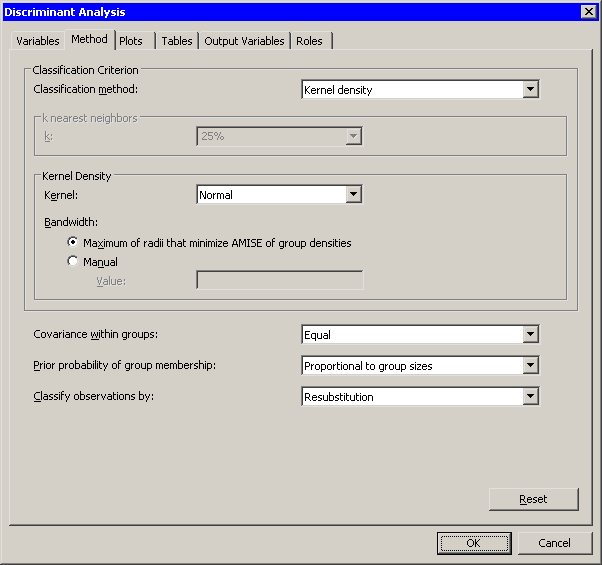
Figure 30.3: The Method Tab

Click the Plots tab.

The Plots tab (Figure 30.4) becomes active.

Select Classification fit plot.

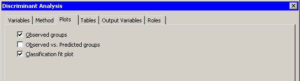
Figure 30.4: The Plots Tab

Click OK.

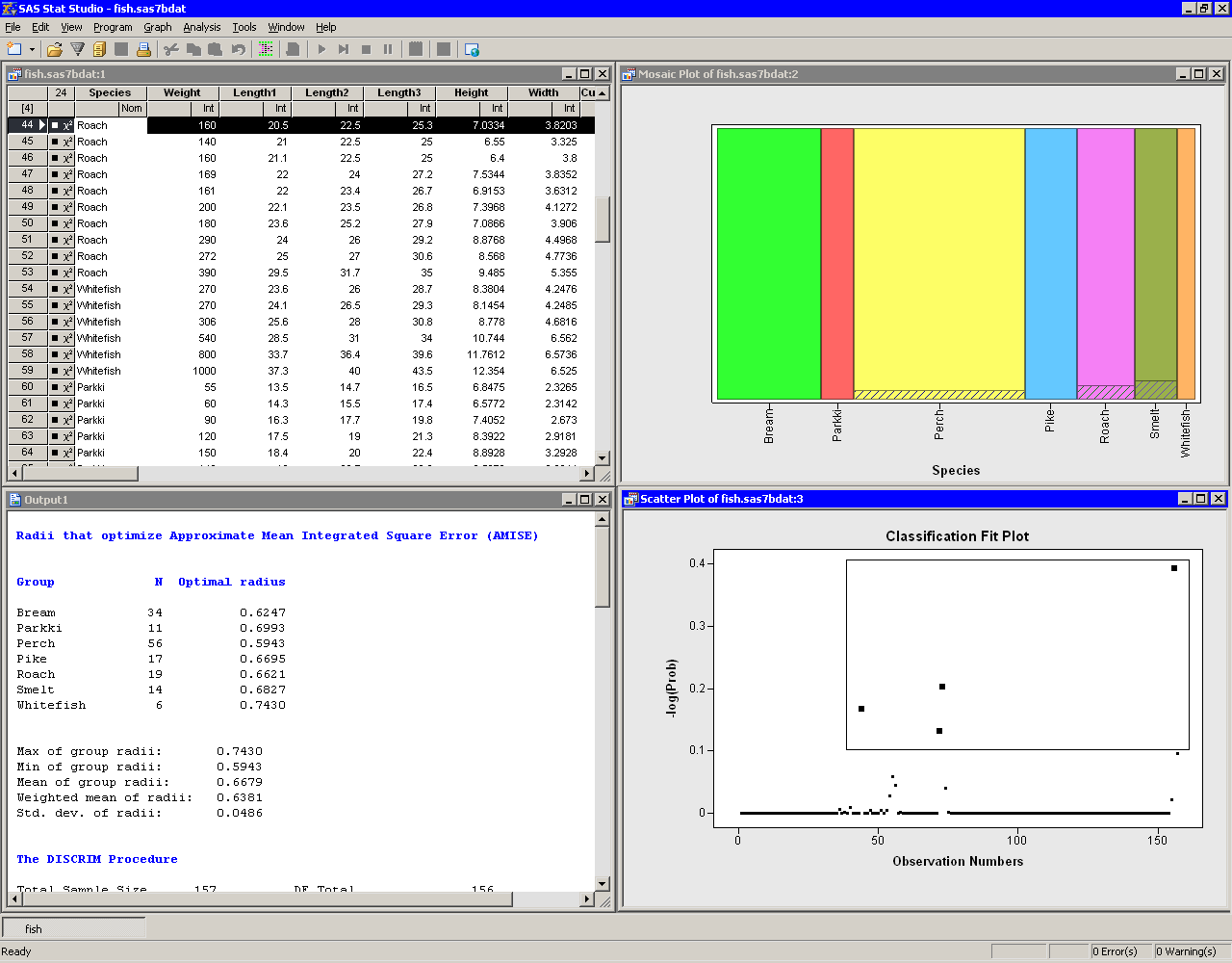
The analysis calls the DISCRIM procedure. The procedure uses the options specified in the dialog box. The procedure displays tables in the output document, as shown in Figure 30.5. Two plots are also created.

Move the classification fit plot so that the workspace is arranged as in Figure 30.5.

The classification fit plot indicates how well each observation is classified by the discriminant function. For each observation, PROC DISCRIM computes posterior probabilities for membership in each group. Let be the maximum posterior probability for the th observation. The classification fit plot is a plot of versus . In Figure 30.5, the selected observations are those with . Equivalently, the maximum posterior probability for membership for the selected observations is less than . The selected fish are those with relatively large probabilities of misclassification. Conversely, selecting the bream, parkki, and pike species in the spine plot (the upper-right plot in Figure 30.5) shows that the classification criterion discriminates between these species quite well. A spine plot is a one-dimensional mosaic plot in which the width of a bar represent the number of observations in a category.

Note: If there are groups, then the maximum posterior probability of membership is at least , so the vertical axis of the classification fit plot is bounded above by .

Figure 30.5: Output from a Discriminant Analysis

The output window contains many tables of statistics. The first table in Figure 30.5 is produced by Stat Studio. It is associated with a heuristic method of choosing the bandwidth for the kernel density classification method. This table is described in the section "The Method Tab".

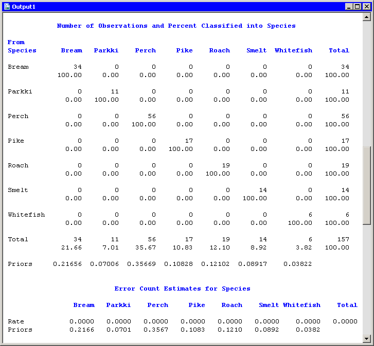
Figure 30.6 displays a table that summarizes how many fish are classified (or misclassified) into each species. If the discriminant function correctly classifies most observations, then the elements on the table's main diagonal are large compared to the off-diagonal elements. For this example, the nonparametric discriminant function correctly classified all fish into the species to which they belong.

Note: The classification in this example was performed using resubstitution. This estimate of the error rate is optimistically biased. You can obtain a less biased estimate by using cross validation. You can select cross validation for the Classify observations by option on the Method tab.

Figure 30.6: Classification of Observations into Groups

In summary, the nonparametric discriminant function in this example does an excellent job of discriminating among these species of fish.