Previous Page

|

Next Page

Modeling the Data

The previous sections describe the Poisson model and create an offset variable for this model. In this section you specify the model.

Select Analysis Model Fitting Generalized Linear Models from the main menu.

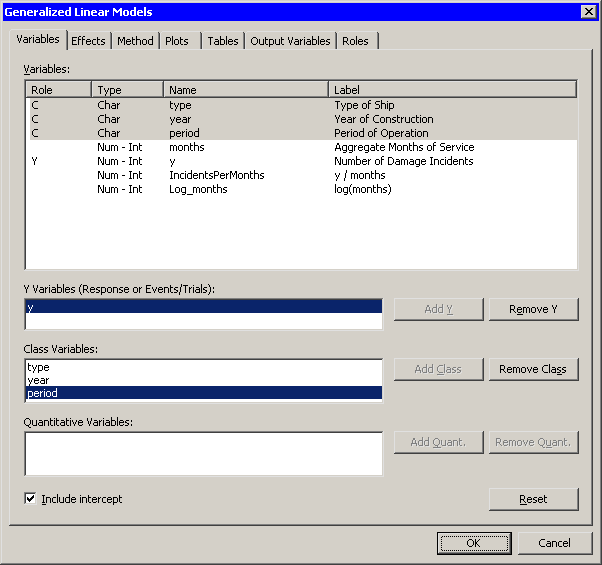
A dialog box appears as in Figure 24.17.

Select y, and click Add Y.

Select type. While holding down the CTRL key, select year, and period. Click Add Class.

Figure 24.17: The Variables Tab

Recall that when you add a variable on the Variables tab, the main effect for that variable is added to the Effects tab. This model includes only the main effects, so you do not need to click the Effects tab.

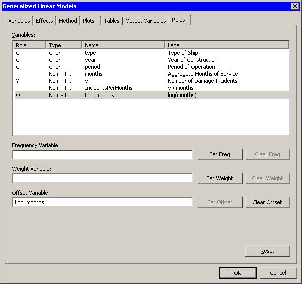
There is one more variable to specify. The following steps specify Log_months as the offset variable:

Click the Roles tab.

The Roles tab appears, as shown in Figure 24.18.

Select Log_months, and click Set Offset.

Figure 24.18: The Roles Tab

You have specified the variables in the model. The next steps specify the response distribution and the link function for a Poisson regression:

Click the Method tab.

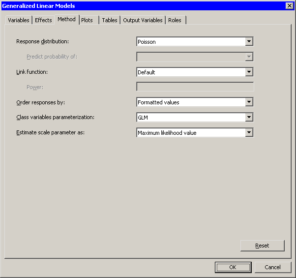
The Method tab appears as in Figure 24.19.

Select Poisson for Response Distribution.

This specifies that the values of y have a probability distribution that is Poisson. (This also implies that the variance of y is proportional to the mean.)

When a response distribution is Poisson, the default link function is the natural log. Consequently, you do not need to change the Link function value.

Figure 24.19: The Method Tab

Click the Tables tab.

The Tables tab becomes active, as shown in Figure 24.9. This tab controls which tables are produced by the analysis.

Clear Wald in the Type 3 Analysis of Contrasts group box.

Select Likelihood Ratio to request statistics for Type 3 contrasts.

Click OK to run the analysis.

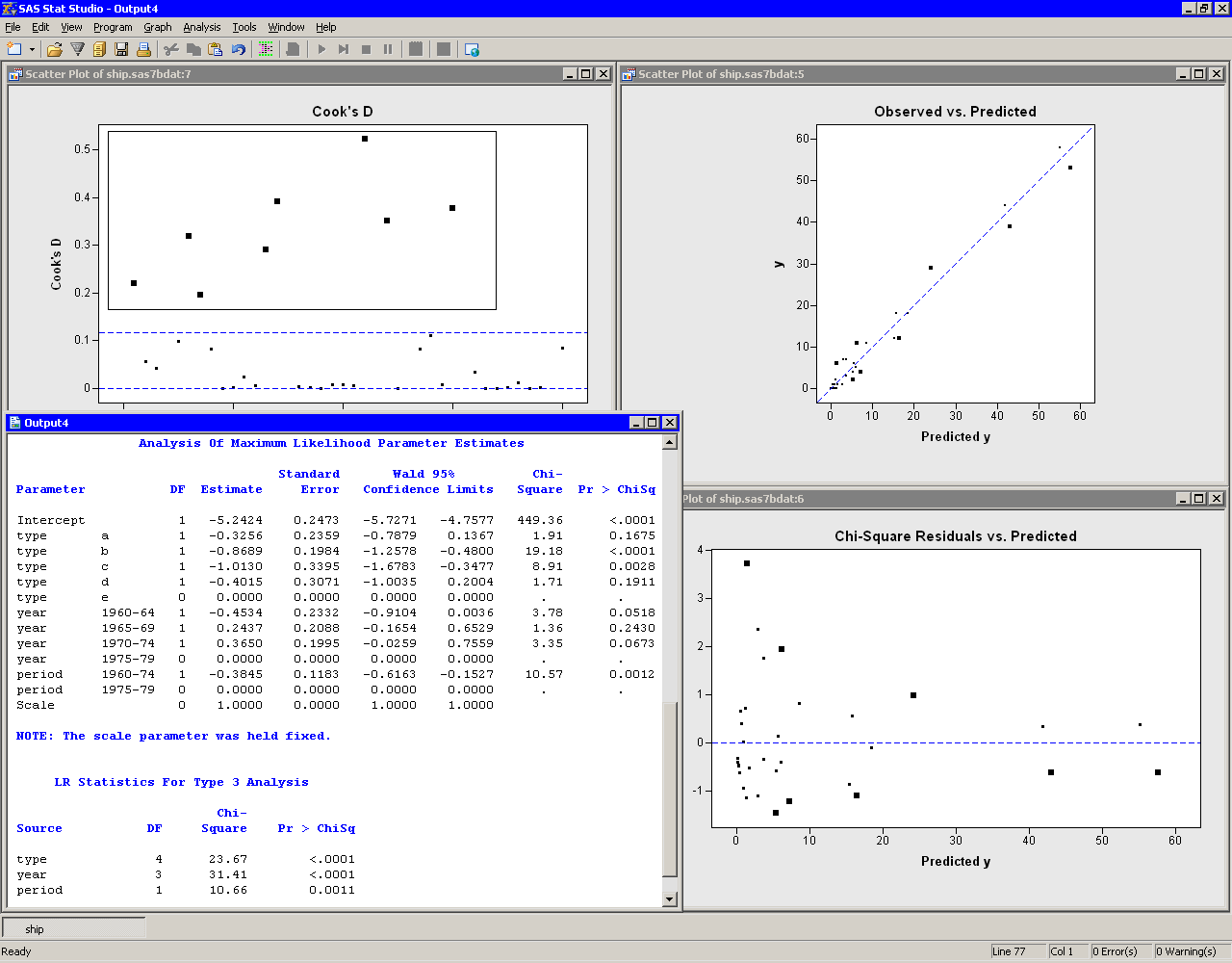
The results of the analysis are shown in Figure 24.20. Move the workspace windows so that they are arranged as in the figure.

The "LR Statistics For Type 3 Analysis" table indicates that all main effects are significant, although period is the weakest of the three.

The "Analysis Of Maximum Likelihood Parameter Estimates" table displays parameter estimates for each level of the effects. The Parameter Estimates column indicates that ships of type b and type c have the lowest risk and ships of type e have the highest. The oldest ships (built from 1960 to 1964) have the lowest risk, and ships built from 1965 to 1974 have the highest risk. However, the estimates of the difference between the older ships and the newer ships are not significantly different from zero (as indicated by the Pr > ChiSq column). Ships operated from 1960 to 1974 have a lower risk than ships operated from 1975 to 1979.

The GENMOD procedure displays a note indicating that the scale parameter is fixed - that is, not estimated by the iterative fitting process.

There are three plots in Figure 24.20. The scatter plot of Cook's (upper left in Figure 24.20) indicates which observations have a large influence on the parameter estimates. Influential observations are highlighted in all plots. Note that the influential observations are not necessarily those with the largest residual values.

Figure 24.20: A Poisson Regression Analysis