The RSREG Procedure

Suppose you have the following data with two factors and three responses, and you want to find the factor setting that produces responses in a certain region:

data a;
   input x1 x2 y1 y2 y3;
   datalines;
-1      -1         1.8 1.940  3.6398
-1       1         2.6 1.843  4.9123
 1      -1         5.4 1.063  6.0128
 1       1         0.7 1.639  2.3629
 0       0         8.5 0.134  9.0910
 0       0         3.0 0.545  3.7349
 0       0         9.8 0.453 10.4412
 0       0         4.1 1.117  5.0042
 0       0         4.8 1.690  6.6245
 0       0         5.9 1.165  6.9420
 0       0         7.3 1.013  8.7442
 0       0         9.3 1.179 10.2762
 1.4142  0         3.9 0.945  5.0245
-1.4142  0         1.7 0.333  2.4041
 0       1.4142    3.0 1.869  5.2695
 0      -1.4142    5.7 0.099  5.4346
;

You want to find the values of x1 and x2 that maximize y1 subject to y2<2 and y3<y2+y1. The exact answer is not easy to obtain analytically, but you can obtain a practically feasible solution by checking conditions across a grid of values in the range of interest. First, append a grid of factor values to the observed data, with missing values for the responses:

data b;
   set a end=eof;
   output;
   if eof then do;
      y1=.;
      y2=.;
      y3=.;
      do x1=-2 to 2 by .1;
         do x2=-2 to 2 by .1;
            output;
         end;
      end;
   end;
run;

Next, use PROC RSREG to fit a response surface model to the data and to compute predicted values for both the observed data and the grid, putting the predicted values in a data set c:

proc rsreg data=b out=c;
   model y1 y2 y3=x1 x2 / predict;
run;

Finally, find the subset of predicted values that satisfy the constraints, sort by the unconstrained variable, and display the top five predictions:

data d;
   set c;
   if y2<2;
   if y3<y2+y1;

proc sort data=d;
   by descending y1;
run;

data d; set d;
   if (_n_ <= 5);
proc print;
run;

The results are displayed in Figure 99.5. They indicate that optimal values of the factors are around 0.3 for x1 and around –0.5 for x2.

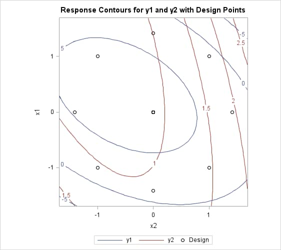
If you are also interested in simultaneously optimizing y1 and y2, you can specify the following statements to make a visual comparison of the two response surfaces by overlaying their contour plots:

ods graphics on;
proc rsreg data=a plots=surface(overlaypairs);
   model y1 y2=x1 x2;
run;
ods graphics off;

Figure 99.6 shows that you have to make some compromises in any attempt to maximize both y1 and y2; however, you might be able to maximize y1 while minimizing y2.

Figure 99.6: Overlaid Line Contours of Predicted Responses