The PRINQUAL Procedure
- Overview
- Getting Started
-
Syntax

-
DetailsThe Three Methods of Variable TransformationUnderstanding How PROC PRINQUAL WorksSplinesMissing ValuesControlling the Number of IterationsPerforming a Principal Component Analysis of Transformed DataUsing the MAC MethodOutput Data SetAvoiding Constant TransformationsConstant VariablesCharacter OPSCORE VariablesREITERATE Option UsagePassive ObservationsComputational ResourcesDisplayed OutputODS Table NamesODS Graphics
-
Examples
- References
Example 92.2 Principal Components of Basketball Rankings
The data in this example are 1985–1986 preseason rankings of 35 U.S. college basketball teams by 10 different news services. The services do not all rank the same teams or the same number of teams, so there are missing values in these data. Each of the 35 teams in the data set is ranked by at least one news service. One way of summarizing these data is with a principal component analysis, since the rankings should all be related to a single underlying variable, the first principal component.
You can use PROC PRINQUAL to estimate the missing ranks and compute scores for all observations. You can formulate a PROC PRINQUAL analysis that assumes that the observed ranks are ordinal variables and replaces the ranks with new numbers that are monotonic with the ranks and better fit the one principal component model. The missing rank estimates need to be constrained since a news service would have positioned the unranked teams below the teams it ranked. PROC PRINQUAL should impose order constraints within the nonmissing values and between the missing and nonmissing values, but not within the missing values. PROC PRINQUAL has sophisticated missing data handling facilities; however, these facilities cannot directly handle this problem. The solution requires reformulating the problem.
By performing some preliminary data manipulations, specifying the N=1 option in the PROC PRINQUAL statement, and specifying the UNTIE transformation in the TRANSFORM statement, you can make the missing value estimates conform to the requirements. The PROC MEANS step finds the largest rank for each variable. The next DATA step replaces missing values with a value that is one larger than the largest observed rank. The PROC PRINQUAL N=1 option specifies that the variables should be transformed to make them as one-dimensional as possible. The UNTIE transformation in the TRANSFORM statement monotonically transforms the ranks, untying any ties in an optimal way. Because the only ties are for the values that replace the missing values, and because these values are larger than the observed values, the rescoring of the data satisfies the preceding requirements.
The following statements create the data set and perform the transformations discussed previously. These statements produce Output 92.2.1 and Output 92.2.2.
*  Preseason 1985 College Basketball Rankings
*  (rankings of 35 teams by 10 news services)
*
*  Note:(a) Various news services rank varying numbers of teams.
*       (b) Not all 35 teams are ranked by all news services.
*       (c) Each team is ranked by at least one service.
*       (d) Rank 20 is missing for UPI.;

title1 '1985 Preseason College Basketball Rankings';

data bballm;
   input School $13. CSN DurhamSun DurhamHerald WashingtonPost
         USA_Today SportMagazine InsideSports UPI AP SportsIllustrated;
   label CSN               = 'Community Sports News (Chapel Hill, NC)'
         DurhamSun         = 'Durham Sun'
         DurhamHerald      = 'Durham Morning Herald'
         WashingtonPost    = 'Washington Post'
         USA_Today         = 'USA Today'
         SportMagazine     = 'Sport Magazine'
         InsideSports      = 'Inside Sports'
         UPI               = 'United Press International'
         AP                = 'Associated Press'
         SportsIllustrated = 'Sports Illustrated'
         ;
   format CSN--SportsIllustrated 5.1;
   datalines;
Louisville     1  8  1  9  8  9  6 10  9  9
Georgia Tech   2  2  4  3  1  1  1  2  1  1
Kansas         3  4  5  1  5 11  8  4  5  7
Michigan       4  5  9  4  2  5  3  1  3  2
Duke           5  6  7  5  4 10  4  5  6  5
UNC            6  1  2  2  3  4  2  3  2  3
Syracuse       7 10  6 11  6  6  5  6  4 10
Notre Dame     8 14 15 13 11 20 18 13 12  .
Kentucky       9 15 16 14 14 19 11 12 11 13
LSU           10  9 13  . 13 15 16  9 14  8
DePaul        11  . 21 15 20  . 19  .  . 19
Georgetown    12  7  8  6  9  2  9  8  8  4
Navy          13 20 23 10 18 13 15  . 20  .
Illinois      14  3  3  7  7  3 10  7  7  6
Iowa          15 16  .  . 23  .  . 14  . 20
Arkansas      16  .  .  . 25  .  .  .  . 16
Memphis State 17  . 11  . 16  8 20  . 15 12
Washington    18  .  .  .  .  .  . 17  .  .
UAB           19 13 10  . 12 17  . 16 16 15
UNLV          20 18 18 19 22  . 14 18 18  .
NC State      21 17 14 16 15  . 12 15 17 18
Maryland      22  .  .  . 19  .  .  . 19 14
Pittsburgh    23  .  .  .  .  .  .  .  .  .
Oklahoma      24 19 17 17 17 12 17  . 13 17
Indiana       25 12 20 18 21  .  .  .  .  .
Virginia      26  . 22  .  . 18  .  .  .  .
Old Dominion  27  .  .  .  .  .  .  .  .  .
Auburn        28 11 12  8 10  7  7 11 10 11
St. Johns     29  .  .  .  . 14  .  .  .  .
UCLA          30  .  .  .  .  .  . 19  .  .
St. Joseph's   .  . 19  .  .  .  .  .  .  .
Tennessee      .  . 24  .  . 16  .  .  .  .
Montana        .  .  . 20  .  .  .  .  .  .
Houston        .  .  .  . 24  .  .  .  .  .
Virginia Tech  .  .  .  .  .  . 13  .  .  .
;
* Find maximum rank for each news service and replace
* each missing value with the next highest rank.;

proc means data=bballm noprint;
   output out=maxrank
      max=mcsn mdurs mdurh mwas musa mspom mins mupi map mspoi;
run;

data bball;
   set bballm;
   if _n_=1 then set maxrank;
   array services[10] CSN--SportsIllustrated;
   array maxranks[10] mcsn--mspoi;
   keep School CSN--SportsIllustrated;
   do i=1 to 10;
      if services[i]=. then services[i]=maxranks[i]+1;
   end;
run;

* Assume that the ranks are ordinal and that unranked teams would have
* been ranked lower than ranked teams.  Monotonically transform all ranked
* teams while estimating the unranked teams.  Enforce the constraint that
* the missing ranks are estimated to be less than the observed ranks.
* Order the unranked teams optimally within this constraint.  Do this so
* as to maximize the variance accounted for by one linear combination.
* This makes the data as nearly rank one as possible, given the constraints.
*
* NOTE: The UNTIE transformation should be used with caution.
* It frequently produces degenerate results.;
ods graphics on;

proc prinqual data=bball out=tbball scores n=1 tstandard=z
   plots=transformations;
   title2 'Optimal Monotonic Transformation of Ranked Teams';
   title3 'with Constrained Estimation of Unranked Teams';
   transform untie(CSN -- SportsIllustrated);
   id School;
run;
Output 92.2.1: PRINQUAL Iteration History
| 1985 Preseason College Basketball Rankings |
| Optimal Monotonic Transformation of Ranked Teams |
| with Constrained Estimation of Unranked Teams |
| PRINQUAL MTV Algorithm Iteration History | |||||
|---|---|---|---|---|---|
| Iteration Number |
Average Change |
Maximum Change |
Proportion of Variance |
Criterion Change |
Note |
| 1 | 0.18563 | 0.76531 | 0.85850 | ||
| 2 | 0.03225 | 0.14627 | 0.94362 | 0.08512 | |
| 3 | 0.02126 | 0.10530 | 0.94669 | 0.00307 | |
| 4 | 0.01467 | 0.07526 | 0.94801 | 0.00132 | |
| 5 | 0.01067 | 0.05282 | 0.94865 | 0.00064 | |
| 6 | 0.00800 | 0.03669 | 0.94899 | 0.00034 | |
| 7 | 0.00617 | 0.02862 | 0.94919 | 0.00020 | |
| 8 | 0.00486 | 0.02636 | 0.94932 | 0.00013 | |
| 9 | 0.00395 | 0.02453 | 0.94941 | 0.00009 | |
| 10 | 0.00327 | 0.02300 | 0.94947 | 0.00006 | |
| 11 | 0.00275 | 0.02166 | 0.94952 | 0.00005 | |
| 12 | 0.00236 | 0.02041 | 0.94956 | 0.00004 | |
| 13 | 0.00205 | 0.01927 | 0.94959 | 0.00003 | |
| 14 | 0.00181 | 0.01818 | 0.94962 | 0.00003 | |
| 15 | 0.00162 | 0.01719 | 0.94964 | 0.00002 | |
| 16 | 0.00147 | 0.01629 | 0.94966 | 0.00002 | |
| 17 | 0.00136 | 0.01546 | 0.94968 | 0.00002 | |
| 18 | 0.00128 | 0.01469 | 0.94970 | 0.00002 | |
| 19 | 0.00121 | 0.01398 | 0.94971 | 0.00001 | |
| 20 | 0.00115 | 0.01332 | 0.94973 | 0.00001 | |
| 21 | 0.00111 | 0.01271 | 0.94974 | 0.00001 | |
| 22 | 0.00105 | 0.01213 | 0.94975 | 0.00001 | |
| 23 | 0.00099 | 0.01155 | 0.94976 | 0.00001 | |
| 24 | 0.00095 | 0.01095 | 0.94977 | 0.00001 | |
| 25 | 0.00091 | 0.01038 | 0.94978 | 0.00001 | |
| 26 | 0.00088 | 0.00986 | 0.94978 | 0.00001 | |
| 27 | 0.00084 | 0.00936 | 0.94979 | 0.00001 | |
| 28 | 0.00081 | 0.00889 | 0.94980 | 0.00001 | |
| 29 | 0.00077 | 0.00846 | 0.94980 | 0.00000 | |
| 30 | 0.00073 | 0.00805 | 0.94980 | 0.00000 | Not Converged |
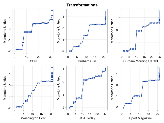
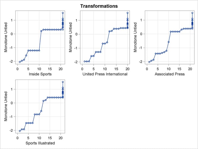
Output 92.2.2: Transformations
An alternative approach is to use the pairwise deletion option of the CORR procedure to compute the correlation matrix and then use PROC PRINCOMP or PROC FACTOR to perform the principal component analysis. This approach has several disadvantages. The correlation matrix might not be positive semidefinite (PSD), an assumption required for principal component analysis. PROC PRINQUAL always produces a PSD correlation matrix. Even with pairwise deletion, PROC CORR removes the six observations that have only a single nonmissing value from this data set. Finally, it is still not possible to calculate scores on the principal components for those teams that have missing values.
You can compute the composite ranking by using PROC PRINCOMP and some preliminary data manipulations, similar to those discussed previously.
Chapter 91: The PRINCOMP Procedure, contains an example where the average of the unused ranks in each poll is substituted for the missing values, and each observation is weighted by the number of nonmissing values. This method has much to recommend it. It is much faster and simpler than using PROC PRINQUAL. It is also much less prone to degeneracies and capitalization on chance. However, PROC PRINCOMP does not allow the nonmissing ranks to be monotonically transformed and the missing values untied to optimize fit.
PROC PRINQUAL monotonically transforms the observed ranks and estimates the missing ranks (within the constraints given previously) to account for almost 95 percent of the variance of the transformed data by just one dimension. PROC FACTOR is then used to report details of the principal component analysis of the transformed data. As shown by the Factor Pattern values in Output 92.2.3, nine of the ten news services have a correlation of 0.95 or larger with the scores on the first principal component after the data are optimally transformed. The scores are sorted and the composite ranking is displayed following the PROC FACTOR output. More confidence can be placed in the stability of the scores for teams that are ranked by the majority of the news services than in scores for teams that are seldom ranked.
The monotonic transformations are plotted for each of the ten news services. See Output 92.2.2. These plots show the values of the raw ranks (with the missing ranks replaced by the maximum rank plus one) versus the rescored (transformed) ranks. The transformations are the step functions that maximize the fit of the data to the principal component model. Smoother transformations could be found by using MSPLINE transformations, but MSPLINE transformations would not correctly handle the missing data problem.
The following statements perform the final analysis and produce Output 92.2.3:
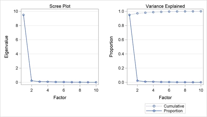
* Perform the Final Principal Component Analysis;
proc factor nfactors=1 plots=scree;
   title4 'Principal Component Analysis';
   ods select factorpattern screeplot;
   var TCSN -- TSportsIllustrated;
run;

proc sort;
   by Prin1;
run;

* Display Scores on the First Principal Component;
proc print;
   title4 'Teams Ordered by Scores on First Principal Component';
   var School Prin1;
run;
Output 92.2.3: Principal Components of College Basketball Rankings
| Factor Pattern | ||
|---|---|---|
| Factor1 | ||
| TCSN | CSN Transformation | 0.91136 |
| TDurhamSun | DurhamSun Transformation | 0.98887 |
| TDurhamHerald | DurhamHerald Transformation | 0.97402 |
| TWashingtonPost | WashingtonPost Transformation | 0.97408 |
| TUSA_Today | USA_Today Transformation | 0.98867 |
| TSportMagazine | SportMagazine Transformation | 0.95331 |
| TInsideSports | InsideSports Transformation | 0.98521 |
| TUPI | UPI Transformation | 0.98534 |
| TAP | AP Transformation | 0.99590 |
| TSportsIllustrated | SportsIllustrated Transformation | 0.98615 |
| 1985 Preseason College Basketball Rankings |
| Optimal Monotonic Transformation of Ranked Teams |
| with Constrained Estimation of Unranked Teams |
| Teams Ordered by Scores on First Principal Component |
| Obs | School | Prin1 |
|---|---|---|
| 1 | Georgia Tech | -6.20315 |
| 2 | UNC | -5.93314 |
| 3 | Michigan | -5.71034 |
| 4 | Kansas | -4.78699 |
| 5 | Duke | -4.75896 |
| 6 | Illinois | -4.19220 |
| 7 | Georgetown | -4.02861 |
| 8 | Louisville | -3.73087 |
| 9 | Syracuse | -3.47497 |
| 10 | Auburn | -1.78429 |
| 11 | LSU | -0.35928 |
| 12 | Memphis State | 0.46737 |
| 13 | Kentucky | 0.63661 |
| 14 | Notre Dame | 0.71919 |
| 15 | Navy | 0.76187 |
| 16 | UAB | 0.98316 |
| 17 | DePaul | 1.09891 |
| 18 | Oklahoma | 1.12012 |
| 19 | NC State | 1.15144 |
| 20 | UNLV | 1.28766 |
| 21 | Iowa | 1.45260 |
| 22 | Indiana | 1.48123 |
| 23 | Maryland | 1.54935 |
| 24 | Virginia | 2.01385 |
| 25 | Arkansas | 2.02718 |
| 26 | Washington | 2.10878 |
| 27 | Tennessee | 2.27770 |
| 28 | Virginia Tech | 2.36103 |
| 29 | St. Johns | 2.37387 |
| 30 | Montana | 2.43502 |
| 31 | UCLA | 2.52481 |
| 32 | Pittsburgh | 3.00907 |
| 33 | Old Dominion | 3.03324 |
| 34 | St. Joseph's | 3.39259 |
| 35 | Houston | 4.69614 |
The ordinary PROC PRINQUAL missing data handling facilities do not work for these data because they do not constrain the missing data estimates properly. If you code the missing ranks as missing and specify linear transformations, then you can compute least squares estimates of the missing values without transforming the observed values. The first principal component then accounts for 92 percent of the variance after 20 iterations. However, Virginia Tech is ranked number 11 by its score even though it appeared in only one poll (Inside Sports ranked it number 13, anchoring it firmly in the middle). Specifying monotone transformations is also inappropriate since they too allow unranked teams to move in between ranked teams.
With these data, the combination of monotone transformations and the freedom to score the missing ranks without constraint leads to degenerate transformations. PROC PRINQUAL tries to merge the 35 points into two points, producing a perfect fit in one dimension. There is evidence for this after 20 iterations when the Average Change, Maximum Change, and Criterion Change values are all increasing, instead of the more stable decreasing change rate seen in the analysis shown. The change rates all stop increasing after 41 iterations, and it is clear by 70 or 80 iterations that one component will account for 100 percent of the transformed variables variance after sufficient iteration. While this might seem desirable (after all, it is a perfect fit), you should, in fact, be on guard when this happens. Whenever convergence is slow, the rates of change increase, or the final data perfectly fit the model, the solution is probably degenerating because of too few constraints on the scorings.
PROC PRINQUAL can account for 100 percent of the variance by scoring Montana and UCLA with one positive value on all variables and scoring all the other teams with one negative value on all variables. This inappropriate analysis suggests that all ranked teams are equally good except for two teams that are less good. Both of these two teams are ranked by only one news service, and their only nonmissing rank is last in the poll. This accounts for the degeneracy.