The MDS Procedure

Formulas
The following notation is used:


-
slope for partition p

-
power for partition p

-
distance computed from the model between objects r and c for subject s

-
data weight for objects r and c for subject s obtained from the cth WEIGHT variable, or 1 if there is no WEIGHT statement
- f
-
value of the FIT= option
- N
-
number of objects

-
observed dissimilarity between objects r and c for subject s

-
partition index for objects r and c for subject s

-
dissimilarity after applying any applicable estimated transformation for objects r and c for subject s


-
standardization factor for partition p

-
estimated transformation for partition p

-
coefficient for subject s on dimension d

-
coordinate for object n on dimension d
Summations are taken over nonmissing values.
Distances are computed from the model as
![\[ D_{rcs} = \begin{cases} \sqrt {\sum _ d(X_{rd}-X_{cd})^2} & \mbox{for COEF=IDENTITY:}\\ & \text {Euclidean distance}\\[2ex] \sqrt {\sum _ d V_{sd}^2(X_{rd}-X_{cd})^2}& \mbox{for COEF=DIAGONAL:}\\ & \text {weighted Euclidean distance} \end{cases} \]](images/statug_mds0025.png)
![\[ \begin{array}{llll} P_{rcs} & = & 1 & \mbox{for CONDITION=UN} \\ & = & s & \mbox{for CONDITION=MATRIX} \\ & = & (s-1)N+r & \mbox{for CONDITION=ROW} \end{array} \]](images/statug_mds0026.png)
The estimated transformation for each partition is
![\[ \begin{array}{llll} T_ p(d) & = & d & \mbox{for LEVEL=ABSOLUTE} \\ & = & B_ pd & \mbox{for LEVEL=RATIO} \\ & = & A_ p+B_ pd & \mbox{for LEVEL=INTERVAL} \\ & = & B_ pd^{C_ p} & \mbox{for LEVEL=LOGINTERVAL} \end{array} \]](images/statug_mds0027.png)
For LEVEL=ORDINAL, is computed as a least-squares monotone transformation.
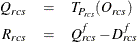
For LEVEL=ABSOLUTE, RATIO, or INTERVAL, the residuals are computed as
![\begin{eqnarray*} Q_{rcs} & =& O_{rcs} \\ R_{rcs} & =& Q_{rcs}^ f - [T_{P_{rcs}}(D_{rcs})]^ f \end{eqnarray*}](images/statug_mds0028.png)
For LEVEL=ORDINAL, the residuals are computed as
If f is 0, then natural logarithms are used in place of the fth powers.
For each partition, let
![\[ U_ p = \frac{\displaystyle {\sum _{r,c,s}F_{rcs}}}{\displaystyle {\sum _{r,c,s | P_{rcs}=p}F_{rcs}}} \]](images/statug_mds0030.png)
and
![\[ \overline{Q}_ p = \frac{\displaystyle {\sum _{r,c,s | P_{rcs}=p}Q_{rcs}F_{rcs}}}{\displaystyle {\sum _{r,c,s | P_{rcs}=p}F_{rcs}}} \]](images/statug_mds0031.png)
Then the standardization factor for each partition is
![\[ \begin{array}{llll} S_ p & =& 1 & \mbox{for FORMULA=0} \\ & =& U_ p \displaystyle {\sum _{r,c,s | P_{rcs}=p} Q_{rcs}^2F_{rcs} } & \mbox{for FORMULA=1} \\ & =& U_ p \displaystyle {\sum _{r,c,s | P_{rcs}=p} (Q_{rcs}-\overline{Q}_ p)^2F_{rcs} } & \mbox{for FORMULA=2} \end{array} \]](images/statug_mds0032.png)
The badness-of-fit criterion that the MDS procedure tries to minimize is
![\[ \sqrt {\displaystyle {\sum _{r,c,s} \frac{R_{rcs}^2 F_{rcs} }{S_{P_{rcs}}} } } \]](images/statug_mds0033.png)