The KRIGE2D Procedure

The Nugget Effect

For all the semivariogram models considered previously, the following property holds:

$\gamma _ z(0) = \lim _{h \downarrow 0}\gamma _ z(h) = 0$

However, a plot of the experimental semivariogram might indicate a discontinuity at h = 0; that is, $\gamma _ z(h) \rightarrow c_ n > 0$ as $h \rightarrow 0$ , while $\gamma _ z(0)=0$ . The quantity $c_ n$ is called the nugget effect; this term is from mining geostatistics where nuggets literally exist, and it represents variations at a much smaller scale than any of the measured pairwise distances—that is, at distances $h \ll h_{\mathit{min}}$ , where

$h_{\mathit{min}} = \min _{i,j}{h_{ij}}= \min _{i,j}{\mid \bm {s}_ i-\bm {s}_ j\mid }$

Nonzero nugget effects have been associated with conceptual and theoretical difficulties; see Cressie (1993, section 2.3.1) and Christakos (1992, section 7.4.3) for details. There is no practical difficulty, however; you simply visually extrapolate the experimental semivariogram as $h \rightarrow 0$ . The importance of availability of data at small lag distances is again illustrated.

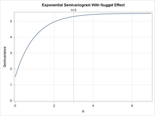
As an example, an exponential semivariogram with a nugget effect $c_ n$ has the form

$\gamma _ z(h) = c_ n + {\sigma _0}^2\left[1-\exp \left(-\frac{h}{a_0}\right)\right], h > 0$

and

$\gamma _ z(0) = 0$

where the factor ${\sigma _0}^2$ is called the partial sill and the sill $c_0 = c_ n + {\sigma _0}^2$ .

This is illustrated in Figure 67.11 for the parameters $a_0=1$ , ${\sigma _0}^2=4$ , and nugget effect $c_ n=1.5$ .

You can specify the nugget effect in PROC KRIGE2D with the NUGGET= option in the MODEL statement. It is a separate, additive term independent of direction; that is, it is isotropic. The way to approximate an anisotropic nugget effect is described in the following section.

Figure 67.11: Exponential Semivariogram Model with a Nugget Effect $c_ n=1.5$