Introduction to Structural Equation Modeling with Latent Variables

Sections Errors-in-Variables Regression, Regression with Measurement Errors in X and Y, and Illustration of Model Identification: Spleen Data show how you can specify models by means of equations in the LINEQS modeling language. This section shows you how to specify models that are represented by path diagrams. The PATH modeling language of PROC CALIS is the main tool for this purpose.

Complicated models are often easier to understand when they are expressed as path diagrams. One advantage of path diagrams over equations is that variances and covariances can be shown directly in the path diagram. Loehlin (1987) provides a detailed discussion of path diagrams. Another advantage is that the path diagram can be transcribed easily into the PATH modeling language supported by PROC CALIS.

A path diagram for the spleen data is shown in Figure 17.13. It explicitly shows all latent variables (including error terms) and variances of exogenous variables.

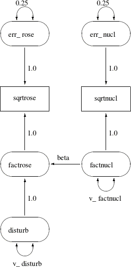
The path diagram shown in Figure 17.13 is essentially a graphical representation of the same just-identified model for the spleen data that is described in the section Illustration of Model Identification: Spleen Data. In path diagrams, it is customary to write the names of manifest or observed variables in rectangles and the names of latent variables in ovals. For example, sqrtrose and sqrtnucl are observed variables in the path diagram, while all others are latent variables.

The effects (the regression coefficients) in each equation are indicated by drawing arrows from the predictor variables to the outcome variable. For example, the path from factnucl to factrose is labeled with the regression coefficient beta in the path diagram shown in Figure 17.13. Other paths are labeled with fixed coefficients (or effects) of 1.

Variances of exogenous variables are drawn as double-headed arrows in Figure 17.13. For example, the variance of disturb is shown as a double-headed arrow pointing to the variable itself and is named v_disturb. Variances of the err_nucl and err_rose are also drawn as double-headed arrows but are labeled with fixed constants 0.25.

The path diagram shown in Figure 17.13 matches the features in the LINEQS model closely. For example, the error terms are depicted explicitly and their paths (regression coefficients) that connect to the associated endogenous variables are marked with fixed constants 1, reflecting the same specification in the equations of the LINEQS model. However, you can simplify the path diagram by using McArdle’s RAM (reticular action model) notation (McArdle and McDonald 1984), as described in the following section.