The ICLIFETEST Procedure

Example 62.1 Analyzing Data with Observations below a Limit of Detection
Data that have certain values below a limit of detection (LOD) are frequently encountered by toxicologists and environmental
scientists. Such data are usually analyzed by imputing the unobserved values by LOD/2 or LOD/ . This type of practice often raises the question of whether the population distributions can be estimated without bias. Gillespie
et al. (2010) propose using a reverse Kaplan-Meier estimator, or equivalently, Turnbull’s method (1976) by treating the unobserved data as left-censored. When the assumption of independent censoring holds, these estimators can
unbiasedly estimate the population distribution functions.
. This type of practice often raises the question of whether the population distributions can be estimated without bias. Gillespie
et al. (2010) propose using a reverse Kaplan-Meier estimator, or equivalently, Turnbull’s method (1976) by treating the unobserved data as left-censored. When the assumption of independent censoring holds, these estimators can
unbiasedly estimate the population distribution functions.
The following hypothetical data have two values, 3 and 10, that are below the limit of detection:
data temp;
   input C1 C2;
   datalines;
  .     3
  4     4
  6     6
  8     8
  .     10
  12    12
;
The following statements invoke PROC ICLIFETEST to estimate the population distribution function by using Turnbull’s method:
proc iclifetest data=temp method=turnbull plots=survival(failure)
                impute(seed=1234);
   time (c1,c2);
run;
Specifying the PLOTS=SURVIVAL(FAILURE) option requests a failure probability plot. Results are shown in Output 62.1.1. Note that because the first Turnbull interval is  , the failure probability function is undefined within that interval.
Output 62.1.1: Failure Probability Plot for Fictitious Nondetection Data
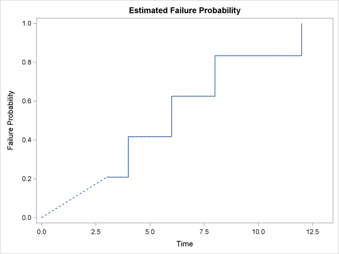
Output 62.1.2 presents the estimated failure probability, with standard errors that are estimated by the method of multiple imputations.
Output 62.1.2: Cumulative Probability Estimates
| Nonparametric Survival Estimates | |||||
|---|---|---|---|---|---|
| Probability Estimate | Imputation Standard Error |
Lagrange Multiplier |
|||
| Time Interval | Failure | Survival | |||
| 3 | 4 | 0.2083 | 0.7917 | 0.1811 | 0.0000 |
| 4 | 6 | 0.4167 | 0.5833 | 0.2179 | 0.0000 |
| 6 | 8 | 0.6250 | 0.3750 | 0.2099 | 0.0000 |
| 8 | 12 | 0.8333 | 0.1667 | 0.1521 | 0.0000 |
| 12 | Inf | 1.0000 | 0.0000 | 0.0000 | 0.0000 |