The VARCOMP Procedure

When no exact confidence limits exist, it is common practice to use approximate confidence limits. Two such approximations are the modified large-sample (MLS) method and the generalized confidence limit (GCL) method as discussed in Burdick, Borror, and Montgomery (2005). When analyzing a balanced one-way or two-way design, if you specify the CL= option with METHOD= TYPE1 or GRR, the VARCOMP procedure computes confidence limits by using either the MLS method (the default) or the GCL method. Generalized confidence limits are obtained by specifying the CL= GCL option in the MODEL statement.
The method of MLS confidence limits was first introduced by Graybill and Wang (1980). It starts with approximate large-sample confidence limits; then it modifies the limits to be exact under certain parameter conditions.
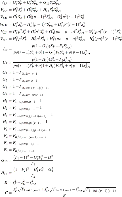
For a balanced two-way crossed random model with interaction, formulas for the MLS method are given in Table 108.6. See Burdick, Borror, and Montgomery (2005) for the formulas for one-way or balanced two-way with no interaction models.
Confidence limits for parameters such as variances and their ratios might not contain the corresponding point estimates, because negative confidence bounds are increased to zero.
The terms in Table 108.6 are defined as follows:
The symbol ![]() represents the percentile of an F distribution with df1 and df2 degrees of freedom and area
represents the percentile of an F distribution with df1 and df2 degrees of freedom and area ![]() to the left.
to the left.
The method of generalized confidence limits was first introduced by Weerahandi (1993). The 100(1-![]() )% generalized confidence limits are determined as follows:
)% generalized confidence limits are determined as follows:
-
Initialize the random number generator with the seed. The seed value is specified by the SEED= option.
-
Sample N generalized pivot quantities (GPQ), defined to have a distribution that is independent of the parameters under study. The value N is specified by the NSAMPLE= option.
-
Define the lower and upper limits as the
 and
and  quantiles of the sampled GPQ values.
Formulas for generalized confidence limits are given in Table 108.7, where Z denotes a standard normal random variable and ![]() and
and ![]() denote jointly independent chi-square random variables that are independent of Z with degrees of freedom
denote jointly independent chi-square random variables that are independent of Z with degrees of freedom ![]() and
and ![]() , respectively. The value of
, respectively. The value of ![]() in Table 108.7 is specified by the EPSILON=
option.
in Table 108.7 is specified by the EPSILON=
option.
In general, the GCL method provides a more accurate confidence interval with a shorter interval width than the MLS method. However, the greater accuracy comes at the cost of being somewhat nondeterministic, because of the reliance on simulation.