The SURVEYPHREG Procedure
- Overview
- Getting Started
-
Syntax
 PROC SURVEYPHREG StatementBY StatementCLASS StatementCLUSTER StatementDOMAIN StatementESTIMATE StatementFREQ StatementLSMEANS StatementLSMESTIMATE StatementMODEL StatementNLOPTIONS StatementOUTPUT StatementProgramming StatementsREPWEIGHTS StatementSLICE StatementSTORE StatementSTRATA StatementTEST StatementWEIGHT Statement
 -
Details
 Notation and EstimationFailure Time DistributionTime and CLASS Variables UsagePartial Likelihood Function for the Cox ModelSpecifying the Sample DesignMissing ValuesVariance EstimationDomain AnalysisHypothesis Tests, Confidence Intervals, and ResidualsOutput Data SetsDisplayed OutputODS Table NamesODS Graphics
 -
Examples

- References
This section describes the computation of residuals (RESMART, RESDEV, RESSCH, and RESSCO in the OUTPUT statement). See the section Notation and Estimation for definition of notation that is used in this section. The residuals are calculated based on the TIES= option in the MODEL statement.
This is the default option. Let
where ![]() ; and A be the set of indices in the selected sample.
; and A be the set of indices in the selected sample.
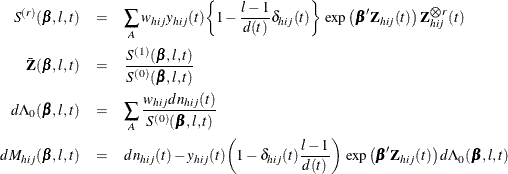
Further let

The martingale residual at t is defined as

Here ![]() estimates the difference over
estimates the difference over ![]() between the observed number of events for the
between the observed number of events for the ![]() observation unit and a conditional expected number of events. The quantity
observation unit and a conditional expected number of events. The quantity ![]() is referred to as the martingale residual for the
is referred to as the martingale residual for the ![]() observation unit. For the Cox model with no time-dependent explanatory variables, the martingale residual for the
observation unit. For the Cox model with no time-dependent explanatory variables, the martingale residual for the ![]() unit with observation time
unit with observation time ![]() and event status
and event status ![]() is
is
The deviance residual ![]() for the
for the ![]() observation unit is a transformation of the corresponding martingale residuals,
observation unit is a transformation of the corresponding martingale residuals,
The square root shrinks large negative martingale residuals, while the logarithmic transformation expands martingale residuals that are close to unity. As such, the deviance residuals are more symmetrically distributed around zero than the martingale residuals. For the Cox model, the deviance residual reduces to the form
The Schoenfeld (1982) residual vector is calculated on a per-event-time basis. At the kth event time ![]() of the
of the ![]() observation unit, the Schoenfeld residual
observation unit, the Schoenfeld residual
is the difference between the observed covariate vector for the ![]() observation unit and the average of the covariate vectors over the risk set at
observation unit and the average of the covariate vectors over the risk set at ![]() . Under the proportional hazards assumption, the Schoenfeld residuals have the sample path of a random walk; therefore, they
are useful in assessing time trend or lack of proportionality.
. Under the proportional hazards assumption, the Schoenfeld residuals have the sample path of a random walk; therefore, they
are useful in assessing time trend or lack of proportionality.
The score process for the ![]() subject at time t is
subject at time t is
The vector ![]() is the score residual for the
is the score residual for the ![]() observation unit.
observation unit.
The score residuals are a decomposition of the first partial derivative of the log likelihood. They are useful in assessing the influence of each subject on individual parameter estimates. They also play an important role in the computation of the variance estimators.
For TIES=EFRON, the preceding computation is modified to comply with the Efron partial likelihood. For a given uncensored
time t, let ![]() if t is an event time for the
if t is an event time for the ![]() observation, and 0 otherwise. Let
observation, and 0 otherwise. Let ![]() , which is the number of observation units that have an event at t. For
, which is the number of observation units that have an event at t. For ![]() , let
, let

where ![]() , and A are the set of indices in the selected sample.
, and A are the set of indices in the selected sample.
The martingale residual at t for the ![]() observation unit is defined as
observation unit is defined as

Deviance residuals are computed by using the same transform on the corresponding martingale residuals as in TIES=BRESLOW.
The Schoenfeld residual vector for the ![]() observation unit at event time
observation unit at event time ![]() is
is
The score process for the ![]() observation unit at time t is
observation unit at time t is