The PLS Procedure

The EFFECT statement makes it easy to construct a wide variety of linear models. In particular, you can use the spline effect to add smoothing terms to a model. A particular benefit of using spline effects in PROC PLS is that, when operating on spline basis functions, the partial least squares algorithm effectively chooses the amount of smoothing automatically, especially if you combine it with cross validation for the selecting the number of factors. This example employs the EFFECT statement to demonstrate partial least squares spline smoothing of agricultural data.
Weibe (1935) presents data from a study of uniformity of wheat yields over a certain rectangular plot of land. The following statements
read these wheat yield measurements, indexed by row and column distances, into the SAS data set Wheat:
data Wheat;
   keep Row Column Yield;
   input Yield @@;
   iRow = int((_N_-1)/12);
   iCol = mod( _N_-1 ,12);
   Column = iCol*15 + 1; /* Column distance, in feet */
   Row    = iRow* 1 + 1; /* Row    distance, in feet */
   Row = 125 - Row + 1;  /* Invert rows              */
   datalines;
 715 595 580 580 615 610 540 515 557 665 560 612
 770 710 655 675 700 690 565 585 550 574 511 618
 760 715 690 690 655 725 665 640 665 705 644 705
 665 615 685 555 585 630 550 520 553 616 573 570
 755 730 670 580 545 620 580 525 495 565 599 612
 745 670 585 560 550 710 590 545 538 587 600 664
 645 690 550 520 450 630 535 505 530 536 611 578
 585 495 455 470 445 555 500 450 420 461 531 559

   ... more lines ...

 570 585 635 765 550 675 765 620 608 705 677 660
 505 500 580 655 470 565 570 555 537 585 589 619
 465 430 510 680 460 600 670 615 620 594 616 784
;
The following statements use the PLS procedure to smooth these wheat yields using two spline effects, one for rows and another
for columns, in addition to their crossproduct. Each spline effect has, by default, seven basis columns; thus their crossproduct
has ![]() columns, for a total of 63 parameters in the full linear model. However, the predictive PLS model does not actually need
to have 63 degrees of freedom. Rather, the degree of smoothing is controlled by the number of PLS factors, which in this case
is chosen automatically by random subset validation with the CV=RANDOM option.
columns, for a total of 63 parameters in the full linear model. However, the predictive PLS model does not actually need
to have 63 degrees of freedom. Rather, the degree of smoothing is controlled by the number of PLS factors, which in this case
is chosen automatically by random subset validation with the CV=RANDOM option.
ods graphics on;

proc pls data=Wheat cv=random(seed=1) cvtest(seed=12345)
         plot(only)=contourfit(obs=gradient);
   effect splCol = spline(Column);
   effect splRow = spline(Row   );
   model Yield = splCol|splRow;
run;
These statements produce the output shown in Output 76.4.1 through Output 76.4.4.
Output 76.4.1: Default Spline Basis: Model and Data Information
| Data Set | WORK.WHEAT |
|---|---|
| Factor Extraction Method | Partial Least Squares |
| PLS Algorithm | NIPALS |
| Number of Response Variables | 1 |
| Number of Predictor Parameters | 63 |
| Missing Value Handling | Exclude |
| Maximum Number of Factors | 15 |
| Validation Method | 10-fold Random Subset Validation |
| Random Subset Seed | 1 |
| Validation Testing Criterion | Prob T**2 > 0.1 |
| Number of Random Permutations | 1000 |
| Random Permutation Seed | 12345 |
Output 76.4.2: Default Spline Basis: Random Subset Validated PRESS Statistics for Number of Factors
| Random Subset Validation for the Number of Extracted Factors |
|||
|---|---|---|---|
| Number of Extracted Factors |
Root Mean PRESS | T**2 | Prob > T**2 |
| 0 | 1.066355 | 251.8793 | <.0001 |
| 1 | 0.826177 | 123.8161 | <.0001 |
| 2 | 0.745877 | 61.6035 | <.0001 |
| 3 | 0.725181 | 44.99644 | <.0001 |
| 4 | 0.701464 | 23.20199 | <.0001 |
| 5 | 0.687164 | 8.369711 | 0.0030 |
| 6 | 0.683917 | 8.775847 | 0.0010 |
| 7 | 0.677969 | 2.907019 | 0.0830 |
| 8 | 0.676423 | 2.190871 | 0.1340 |
| 9 | 0.676966 | 3.191284 | 0.0600 |
| 10 | 0.675026 | 1.334638 | 0.2390 |
| 11 | 0.673906 | 0.556455 | 0.4470 |
| 12 | 0.673653 | 1.257292 | 0.2790 |
| 13 | 0.672669 | 0 | 1.0000 |
| 14 | 0.673596 | 2.386014 | 0.1190 |
| 15 | 0.672828 | 0.02962 | 0.8820 |
Output 76.4.3: Default Spline Basis: PLS Variation Summary for Split-Sample Validated Model
| Percent Variation Accounted for by Partial Least Squares Factors |
||||
|---|---|---|---|---|
| Number of Extracted Factors |
Model Effects | Dependent Variables | ||
| Current | Total | Current | Total | |
| 1 | 11.5269 | 11.5269 | 40.2471 | 40.2471 |
| 2 | 7.2314 | 18.7583 | 10.4908 | 50.7379 |
| 3 | 6.9147 | 25.6730 | 2.6523 | 53.3902 |
| 4 | 3.8433 | 29.5163 | 2.8806 | 56.2708 |
| 5 | 6.4795 | 35.9958 | 1.3197 | 57.5905 |
| 6 | 7.6201 | 43.6159 | 1.1700 | 58.7605 |
| 7 | 7.3214 | 50.9373 | 0.7186 | 59.4790 |
| 8 | 4.8363 | 55.7736 | 0.4548 | 59.9339 |
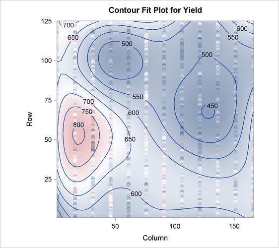
The cross validation results in Output 76.4.2 point to a model with eight PLS factors; this is the smallest model whose predicted residual sum of squares (PRESS) is insignificantly
different from the model with the absolute minimum PRESS. The variation summary in Output 76.4.3 shows that this model accounts for about 60% of the variation in the Yield values. The OBS=GRADIENT suboption for the PLOT=CONTOURFIT option specifies that the observations in the resulting plot,
Output 76.4.4, be colored according to the same scheme as the surface of predicted yield. This coloration enables you to easily tell which
observations are above the surface of predicted yield and which are below.
The surface of predicted yield is somewhat smoother than what Weibe (1935) settled on originally, with a predominance of simple, elliptically shaped contours. You can easily specify a potentially more granular model by increasing the number of knots in the spline bases. Even though the more granular model increases the number of predictor parameters, cross validation can still protect you from overfitting the data. The following statements are the same as those shown before, except that the spline effects now have twice as many basis functions:
ods graphics on;

proc pls data=Wheat cv=random(seed=1) cvtest(seed=12345)
         plot(only)=contourfit(obs=gradient);
   effect splCol = spline(Column / knotmethod=equal(14));
   effect splRow = spline(Row    / knotmethod=equal(14));
   model Yield = splCol|splRow;
run;
The resulting output is shown in Output 76.4.5 through Output 76.4.8.
Output 76.4.5: More Granular Spline Basis: Model and Data Information
| Data Set | WORK.WHEAT |
|---|---|
| Factor Extraction Method | Partial Least Squares |
| PLS Algorithm | NIPALS |
| Number of Response Variables | 1 |
| Number of Predictor Parameters | 360 |
| Missing Value Handling | Exclude |
| Maximum Number of Factors | 15 |
| Validation Method | 10-fold Random Subset Validation |
| Random Subset Seed | 1 |
| Validation Testing Criterion | Prob T**2 > 0.1 |
| Number of Random Permutations | 1000 |
| Random Permutation Seed | 12345 |
Output 76.4.6: More Granular Spline Basis: Random Subset Validated PRESS Statistics for Number of Factors
| Random Subset Validation for the Number of Extracted Factors |
|||
|---|---|---|---|
| Number of Extracted Factors |
Root Mean PRESS | T**2 | Prob > T**2 |
| 0 | 1.066355 | 247.9268 | <.0001 |
| 1 | 0.652658 | 20.68858 | <.0001 |
| 2 | 0.615087 | 0.074822 | 0.7740 |
| 3 | 0.614128 | 0 | 1.0000 |
| 4 | 0.615268 | 0.197678 | 0.6490 |
| 5 | 0.618001 | 1.372038 | 0.2340 |
| 6 | 0.622949 | 5.035504 | 0.0180 |
| 7 | 0.626482 | 7.296797 | 0.0080 |
| 8 | 0.633316 | 13.66045 | <.0001 |
| 9 | 0.635239 | 16.16922 | <.0001 |
| 10 | 0.636938 | 18.02295 | <.0001 |
| 11 | 0.636494 | 16.9881 | <.0001 |
| 12 | 0.63682 | 16.83341 | <.0001 |
| 13 | 0.637719 | 16.74157 | <.0001 |
| 14 | 0.637627 | 15.79342 | <.0001 |
| 15 | 0.638431 | 16.12327 | <.0001 |
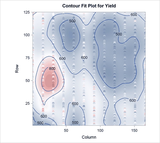
Output 76.4.5 shows that the model now has 360 parameters, many more than before. In Output 76.4.6 you can see that with more granular spline effects, fewer PLS factors are required—only two, in fact. However, Output 76.4.7 shows that this model now accounts for over 70% of the variation in the Yield values, and the contours of predicted values in Output 76.4.8 are less inclined to be simple elliptical shapes.