Introduction to Structural Equation Modeling with Latent Variables

Regression with Measurement Errors in X and Y

What if there are also measurement errors in the outcome variable Y? How can you write such an extended model? The following model would take measurement errors in both X and Y into account:

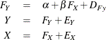
$\begin{eqnarray*} F_ Y & = & \alpha + \beta F_ X + D_{Fy}\nonumber \\ Y & = & F_ Y + E_ Y \nonumber \\ X & = & F_ X + E_ X \nonumber \end{eqnarray*}$

with the following assumption:

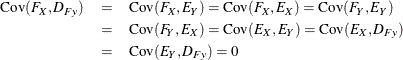
$\begin{eqnarray*} \mbox{Cov}(F_ X,D_{Fy}) & = & \mbox{Cov}(F_ X,E_ Y) = \mbox{Cov}(F_ X,E_ X) = \mbox{Cov}(F_ Y,E_ Y) \\ & = & \mbox{Cov}(F_ Y,E_ X) = \mbox{Cov}(E_ X,E_ Y) = \mbox{Cov}(E_ X,D_{Fy}) \\ & = & \mbox{Cov}(E_ Y,D_{Fy}) = 0 \end{eqnarray*}$

Again, the first equation, expressing the relationship between two latent true-score variables, defines the structural or causal model. The next two equations express the observed variables in terms of a true score plus error; these two equations define the measurement model. This is essentially the same form as the so-called LISREL model (Keesling, 1972; Wiley, 1973; Jöreskog, 1973), which has been popularized by the LISREL program (Jöreskog and Sörbom, 1988). Typically, there are several X and Y variables in a LISREL model. For the moment, however, the focus is on the current regression form in which there is only a single predictor and a single outcome variable. The LISREL model is considered in the section Fitting LISREL Models by the LISMOD Modeling Language.

With the intercept term left out for modeling, you can use the following statements for fitting the regression model with measurement errors in both X and Y:

proc calis data=corn;
   lineqs
      Fy  = beta * Fx + DFy,
      Y   = 1.   * Fy + Ey,
      X   = 1.   * Fx + Ex;
run;

Again, you do not need to specify the zero-correlation assumptions in the LINEQS model because they are set by default given the latent factors and errors in the LINEQS modeling language. When you run this model, PROC CALIS issues the following warning:

   WARNING: Estimation problem not identified: More parameters to 
            estimate ( 5 ) than the total number of mean and 
            covariance elements ( 3 ).

The five parameters in the model include beta and the variances for the exogenous variables: Fx, DFy, Ey, and Ex. These variance parameters are treated as free parameters by default in PROC CALIS. You have five parameters to estimate, but the information for estimating these five parameters comes from the three unique elements in the sample covariance matrix for X and Y. Hence, your model is in the so-called underidentification situation. Model identification is discussed in more detail in the section Model Identification.

To make the current model identified, you can put constraints on some parameters. This reduces the number of independent parameters to estimate in the model. In the errors-in-variables model for the corn data, the variance of Ex (measurement error for X) is given as the constant value 57, which was obtained from a previous study. This could still be applied in the current model with measurement errors in both X and Y. In addition, if you are willing to accept the assumption that the structural equation model is (almost) deterministic, then the variance of Dfy could be set to 0. With these two parameter constraints, the current model is just-identified. That is, you can now estimate three free parameters from three distinct covariance elements in the data. The following statements show the LINEQS model specification for this just-identified model:

proc calis data=corn;
   lineqs
      Fy  = beta * Fx + Dfy,
      Y   = 1.   * Fy + Ey,
      X   = 1.   * Fx + Ex;
   variance
      Ex  = 57.,
      Dfy = 0.;
run;

Figure 17.6 shows the estimation results.

Figure 17.6: Regression Model With Measurement Errors in X and Y for Corn Data

Linear Equations
Fy	=	0.4232	(**)	Fx	+	1.0000	Dfy
y	=	1.0000		Fy	+	1.0000	Ey
x	=	1.0000		Fx	+	1.0000	Ex

Effects in Linear Equations
Variable	Predictor	Parameter	Estimate	Standard Error	t Value	Pr > \|t\|
Fy	Fx	beta	0.42316	0.16582	2.5520	0.0107
y	Fy		1.00000
x	Fx		1.00000

Estimates for Variances of Exogenous Variables
Variable Type	Variable	Parameter	Estimate	Standard Error	t Value	Pr > \|t\|
Error	Ex		57.00000
Disturbance	Dfy		0
Latent	Fx	_Add1	247.85450	136.33508	1.8180	0.0691
Error	Ey	_Add2	43.29105	23.92488	1.8095	0.0704

In Figure 17.6, the estimate of beta is 0.4232, which is basically the same as the estimate for beta in the errors-in-variables model shown in Figure 17.4. The estimated variances for Fx and Ey match for the two models too. In fact, it is not difficult to show mathematically that the current constrained model with measurements errors in both Y and X is equivalent to the errors-in-variables model for the corn data. The numerical results merely confirm this fact.

It is important to emphasize that the equivalence shown here is not a general statement about the current model with measurement errors in X and Y and the errors-in-variables model. Essentially, the equivalence of the two models as applied to the corn data is due to those constraints imposed on the measurement error variances for DFy and Ex. The more important implication from these two analyses is that for the model with measurement errors in both X and Y, you need to set more parameter constraints to make the model identified. Some constraints might be substantively meaningful, while others might need strong or risky assumptions.

For example, setting the variance of Ex to 57 is substantively meaningful because it is based on a prior study. However, setting the variance of Dfy to 0 implies the acceptance of the deterministic structural model, which could be a rather risky assumption in most practical situations. It turns out that using these two constraints together for the model identification of the regression with measurement errors in both X and Y does not give you more substantively important information than what the errors-in-variables model has already given you (compare Figure 17.6 with Figure 17.4). Therefore, the set of identification constraints you use might be important in at least two aspects. First, it might lead to an identified model if you set them properly. Second, given that the model is identified, the meaningfulness of your model depends on how reasonable your identification constraints are.

The two identification constraints set on the regression model with measurement errors in both X and Y make the model identified. But they do not lead to model estimates that are more informative than that of the errors-in-variables regression. Some other sets of identification constraints, if available, might have been more informative. For example, if there were a prior study about the measurement error variance of corn yields (Y), a fixed constant for the variance of Ey could have been set, instead of the unrealistic zero variance constraint of Dfy. This way the estimation results of the regression model with measurement errors in both X and Y would offer you something different from the errors-in-variables regression.

Setting identification constraints could be based on convention or other arguments. See the section Illustration of Model Identification: Spleen Data for an example where model identification is attained by setting constant error variances for X and Y in the model. For the corn data, you have seen that fixing the error variance of the predictor variable led to model identification of the errors-in-variables model. In this case, prior knowledge about the measurement error variance is necessary. This necessity is partly due to the fact that each latent true score variable has only one observed variable as its indicator measure. When you have more measurement indicators for the same latent factor, fixing the measurement error variances to constants for model identification would not be necessary. This is the modeling scenario assumed by the LISREL model (see the section Fitting LISREL Models by the LISMOD Modeling Language), of which the confirmatory factor model is a special case. The confirmatory factor model is described and illustrated in the section The FACTOR and RAM Modeling Languages.