The DISCRIM Procedure

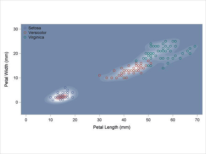
In this example, four more discriminant analyses of iris data are run with two quantitative variables: petal width and petal length. The following statements produce Output 35.2.1 through Output 35.2.5:
title 'Discriminant Analysis of Fisher (1936) Iris Data';
proc template;
define statgraph scatter;
begingraph;
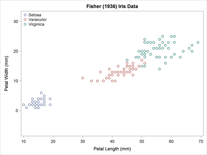
entrytitle 'Fisher (1936) Iris Data';
layout overlayequated / equatetype=fit;
scatterplot x=petallength y=petalwidth /
group=species name='iris';
layout gridded / autoalign=(topleft);
discretelegend 'iris' / border=false opaque=false;
endlayout;
endlayout;
endgraph;
end;
run;
proc sgrender data=sashelp.iris template=scatter;
run;
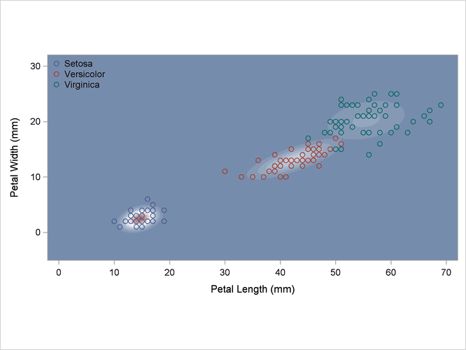
The scatter plot in Output 35.2.1 shows the joint sample distribution.
Another data set is created for plotting, containing a grid of points suitable for contour plots. The following statements create the data set:
data plotdata;
   do PetalLength = -2 to 72 by 0.5;
      do PetalWidth= - 5 to 32 by 0.5;
         output;
      end;
   end;
run;
Three macros are defined as follows to make contour plots of density estimates, posterior probabilities, and classification results:
%let close = thresholdmin=0 thresholdmax=0 offsetmin=0 offsetmax=0;
%let close = xaxisopts=(&close) yaxisopts=(&close);

proc template;
   define statgraph contour;
      begingraph;
         layout overlayequated / equatetype=equate &close;
            contourplotparm x=petallength y=petalwidth z=z /
                            contourtype=fill nhint=30;
            scatterplot x=pl y=pw / group=species name='iris'
                        includemissinggroup=false primary=true;
            layout gridded / autoalign=(topleft);
               discretelegend 'iris' / border=false opaque=false;
            endlayout;
         endlayout;
      endgraph;
   end;
run;

%macro contden;
   data contour(keep=PetalWidth PetalLength species z pl pw);
      merge plotd(in=d) sashelp.iris(keep=PetalWidth PetalLength species
                                     rename=(PetalWidth=pw PetalLength=pl));
      if d then z = max(setosa,versicolor,virginica);
   run;

   title3 'Plot of Estimated Densities';

   proc sgrender data=contour template=contour;
   run;
%mend;

%macro contprob;
   data posterior(keep=PetalWidth PetalLength species z pl pw into);
      merge plotp(in=d) sashelp.iris(keep=PetalWidth PetalLength species
                                     rename=(PetalWidth=pw PetalLength=pl));
      if d then z = max(setosa,versicolor,virginica);
      into = 1 * (_into_ =: 'Set') + 2 * (_into_ =: 'Ver') +
             3 * (_into_ =: 'Vir');
   run;

   title3 'Plot of Posterior Probabilities ';

   proc sgrender data=posterior template=contour;
   run;
%mend;
%macro contclass;
   title3 'Plot of Classification Results';

   proc sgrender data=posterior(drop=z rename=(into=z)) template=contour;
   run;
%mend;
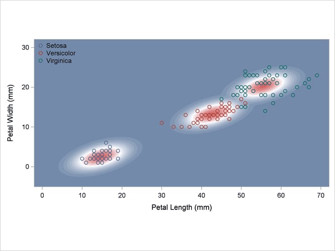
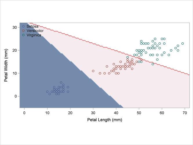
A normal-theory analysis (METHOD=NORMAL) assuming equal covariance matrices (POOL=YES) illustrates the linearity of the classification boundaries. These statements produce Output 35.2.2:
title2 'Using Normal Density Estimates with Equal Variance';

proc discrim data=sashelp.iris method=normal pool=yes
             testdata=plotdata testout=plotp testoutd=plotd
             short noclassify crosslisterr;
   class Species;
   var Petal:;
run;

%contden
%contprob
%contclass
Output 35.2.2: Normal Density Estimates with Equal Variance
| Discriminant Analysis of Fisher (1936) Iris Data |
| Using Normal Density Estimates with Equal Variance |
| Posterior Probability of Membership in Species | ||||||
|---|---|---|---|---|---|---|
| Obs | From Species | Classified into Species |
Setosa | Versicolor | Virginica | |
| 53 | Versicolor | Virginica | * | 0.0000 | 0.2130 | 0.7870 |
| 100 | Versicolor | Virginica | * | 0.0000 | 0.3118 | 0.6882 |
| 103 | Virginica | Versicolor | * | 0.0000 | 0.8453 | 0.1547 |
| 113 | Virginica | Versicolor | * | 0.0000 | 0.8322 | 0.1678 |
| 124 | Virginica | Versicolor | * | 0.0000 | 0.8057 | 0.1943 |
| 136 | Virginica | Versicolor | * | 0.0000 | 0.8903 | 0.1097 |
| * Misclassified observation |
| Discriminant Analysis of Fisher (1936) Iris Data |
| Using Normal Density Estimates with Equal Variance |
| Number of Observations and Percent Classified into Species |
||||||||||||
|---|---|---|---|---|---|---|---|---|---|---|---|---|
| From Species | Setosa | Versicolor | Virginica | Total | ||||||||
| Setosa |
|
|
|
|
||||||||
| Versicolor |
|
|
|
|
||||||||
| Virginica |
|
|
|
|
||||||||
| Total |
|
|
|
|
||||||||
| Priors |
|
|
|
|
||||||||
| Discriminant Analysis of Fisher (1936) Iris Data |
| Using Normal Density Estimates with Equal Variance |
| Observation Profile for Test Data | |
|---|---|
| Number of Observations Read | 11175 |
| Number of Observations Used | 11175 |

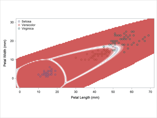
A normal-theory analysis assuming unequal covariance matrices (POOL=NO) illustrates quadratic classification boundaries. These statements produce Output 35.2.3:
title2 'Using Normal Density Estimates with Unequal Variance';

proc discrim data=sashelp.iris method=normal pool=no
             testdata=plotdata testout=plotp testoutd=plotd
             short noclassify crosslisterr;
   class Species;
   var Petal:;
run;

%contden
%contprob
%contclass
Output 35.2.3: Normal Density Estimates with Unequal Variance
| Discriminant Analysis of Fisher (1936) Iris Data |
| Using Normal Density Estimates with Unequal Variance |
| Posterior Probability of Membership in Species | ||||||
|---|---|---|---|---|---|---|
| Obs | From Species | Classified into Species |
Setosa | Versicolor | Virginica | |
| 53 | Versicolor | Virginica | * | 0.0000 | 0.0903 | 0.9097 |
| 100 | Versicolor | Virginica | * | 0.0000 | 0.4675 | 0.5325 |
| 103 | Virginica | Versicolor | * | 0.0000 | 0.7288 | 0.2712 |
| 113 | Virginica | Versicolor | * | 0.0000 | 0.5196 | 0.4804 |
| 136 | Virginica | Versicolor | * | 0.0000 | 0.8335 | 0.1665 |
| * Misclassified observation |
| Discriminant Analysis of Fisher (1936) Iris Data |
| Using Normal Density Estimates with Unequal Variance |
| Number of Observations and Percent Classified into Species |
||||||||||||
|---|---|---|---|---|---|---|---|---|---|---|---|---|
| From Species | Setosa | Versicolor | Virginica | Total | ||||||||
| Setosa |
|
|
|
|
||||||||
| Versicolor |
|
|
|
|
||||||||
| Virginica |
|
|
|
|
||||||||
| Total |
|
|
|
|
||||||||
| Priors |
|
|
|
|
||||||||
| Discriminant Analysis of Fisher (1936) Iris Data |
| Using Normal Density Estimates with Unequal Variance |
| Observation Profile for Test Data | |
|---|---|
| Number of Observations Read | 11175 |
| Number of Observations Used | 11175 |
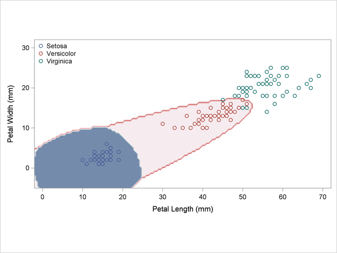
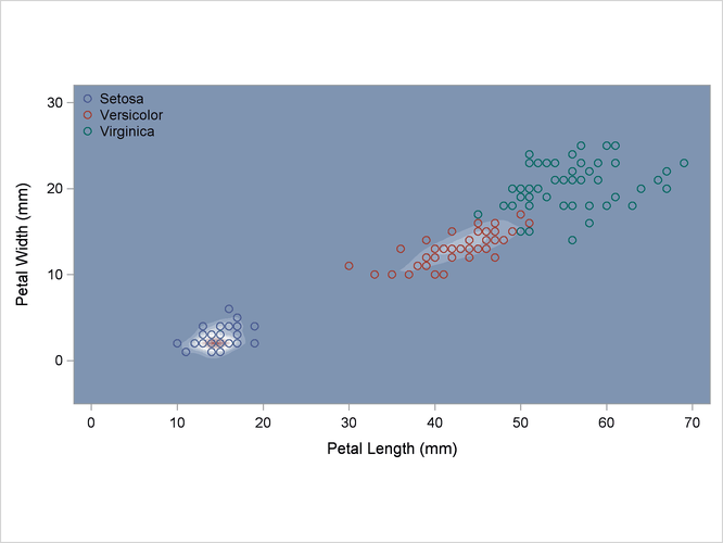
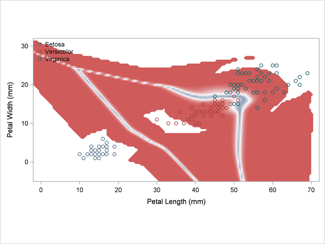
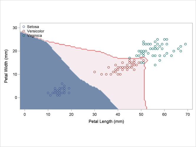
A nonparametric analysis (METHOD=NPAR) follows, using normal kernels (KERNEL=NORMAL) and equal bandwidths (POOL=YES) in each class. The value of the radius parameter r that, assuming normality, minimizes an approximate mean integrated square error is 0.50 (see the section Nonparametric Methods). These statements produce Output 35.2.4:
title2 'Using Kernel Density Estimates with Equal Bandwidth';

proc discrim data=sashelp.iris method=npar kernel=normal
             r=.5 pool=yes testoutd=plotd
             testdata=plotdata testout=plotp
             short noclassify crosslisterr;
   class Species;
   var Petal:;
run;

%contden
%contprob
%contclass
Output 35.2.4: Kernel Density Estimates with Equal Bandwidth
| Discriminant Analysis of Fisher (1936) Iris Data |
| Using Kernel Density Estimates with Equal Bandwidth |
| Posterior Probability of Membership in Species | ||||||
|---|---|---|---|---|---|---|
| Obs | From Species | Classified into Species |
Setosa | Versicolor | Virginica | |
| 53 | Versicolor | Virginica | * | 0.0000 | 0.0800 | 0.9200 |
| 100 | Versicolor | Virginica | * | 0.0000 | 0.4123 | 0.5877 |
| 103 | Virginica | Versicolor | * | 0.0000 | 0.7474 | 0.2526 |
| 113 | Virginica | Versicolor | * | 0.0000 | 0.5863 | 0.4137 |
| 136 | Virginica | Versicolor | * | 0.0000 | 0.8358 | 0.1642 |
| * Misclassified observation |
| Discriminant Analysis of Fisher (1936) Iris Data |
| Using Kernel Density Estimates with Equal Bandwidth |
| Number of Observations and Percent Classified into Species |
||||||||||||
|---|---|---|---|---|---|---|---|---|---|---|---|---|
| From Species | Setosa | Versicolor | Virginica | Total | ||||||||
| Setosa |
|
|
|
|
||||||||
| Versicolor |
|
|
|
|
||||||||
| Virginica |
|
|
|
|
||||||||
| Total |
|
|
|
|
||||||||
| Priors |
|
|
|
|
||||||||
| Discriminant Analysis of Fisher (1936) Iris Data |
| Using Kernel Density Estimates with Equal Bandwidth |
| Observation Profile for Test Data | |
|---|---|
| Number of Observations Read | 11175 |
| Number of Observations Used | 11175 |
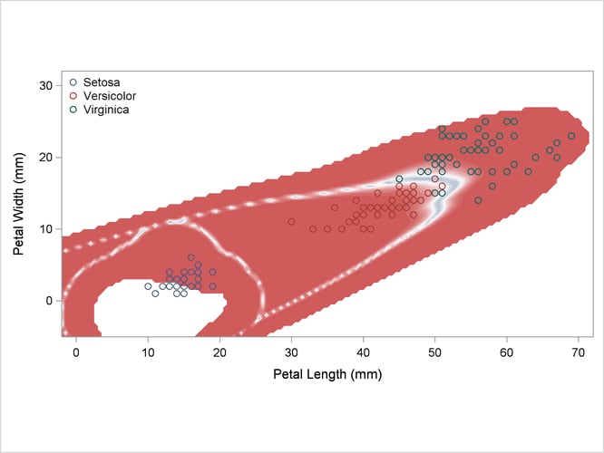
Another nonparametric analysis is run with unequal bandwidths (POOL=NO). These statements produce Output 35.2.5:
title2 'Using Kernel Density Estimates with Unequal Bandwidth';

proc discrim data=sashelp.iris method=npar kernel=normal
             r=.5 pool=no testoutd=plotd
             testdata=plotdata testout=plotp
             short noclassify crosslisterr;
   class Species;
   var Petal:;
run;

%contden
%contprob
%contclass
Output 35.2.5: Kernel Density Estimates with Unequal Bandwidth
| Discriminant Analysis of Fisher (1936) Iris Data |
| Using Kernel Density Estimates with Unequal Bandwidth |
| Posterior Probability of Membership in Species | ||||||
|---|---|---|---|---|---|---|
| Obs | From Species | Classified into Species |
Setosa | Versicolor | Virginica | |
| 53 | Versicolor | Virginica | * | 0.0000 | 0.0516 | 0.9484 |
| 100 | Versicolor | Virginica | * | 0.0000 | 0.3773 | 0.6227 |
| 103 | Virginica | Versicolor | * | 0.0000 | 0.7826 | 0.2174 |
| 136 | Virginica | Versicolor | * | 0.0000 | 0.8802 | 0.1198 |
| * Misclassified observation |
| Discriminant Analysis of Fisher (1936) Iris Data |
| Using Kernel Density Estimates with Unequal Bandwidth |
| Number of Observations and Percent Classified into Species |
||||||||||||
|---|---|---|---|---|---|---|---|---|---|---|---|---|
| From Species | Setosa | Versicolor | Virginica | Total | ||||||||
| Setosa |
|
|
|
|
||||||||
| Versicolor |
|
|
|
|
||||||||
| Virginica |
|
|
|
|
||||||||
| Total |
|
|
|
|
||||||||
| Priors |
|
|
|
|
||||||||
| Discriminant Analysis of Fisher (1936) Iris Data |
| Using Kernel Density Estimates with Unequal Bandwidth |
| Observation Profile for Test Data | |
|---|---|
| Number of Observations Read | 11175 |
| Number of Observations Used | 11175 |