The CLUSTER Procedure

The iris data published by Fisher (1936) have been widely used for examples in discriminant analysis and cluster analysis. The sepal length, sepal width, petal length, and petal width are measured in millimeters on 50 iris specimens from each of three species, Iris setosa, I. versicolor, and I. virginica. Mezzich and Solomon (1980) discuss a variety of cluster analyses of the iris data.
The following step displays the iris SAS data set, which is available in the Sashelp library:
title 'Cluster Analysis of Fisher (1936) Iris Data';

proc print data=sashelp.iris;
run;
The results of this step are not shown.
This example analyzes the iris data by using Ward’s method and two-stage density linkage and then illustrates how the FASTCLUS procedure can be used in combination with PROC CLUSTER to analyze large data sets.
The following macro, SHOW, is used in the subsequent analyses to display cluster results. It invokes the FREQ procedure to crosstabulate clusters and species. The CANDISC procedure computes canonical variables for discriminating among the clusters, and the first two canonical variables are plotted to show cluster membership. See Chapter 31: The CANDISC Procedure, for a canonical discriminant analysis of the iris species.
/*--- Define macro show ---*/
%macro show;
   proc freq;
      tables cluster*species / nopercent norow nocol plot=none;
   run;

   proc candisc noprint out=can;
      class cluster;
      var petal: sepal:;
   run;

   proc sgplot data=can;
      scatter y=can2 x=can1 / group=cluster;
   run;
%mend;
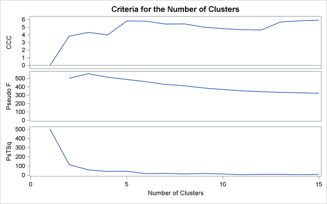
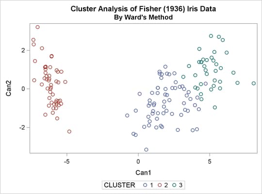
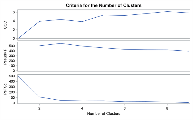
The first analysis clusters the iris data by using Ward’s method (see Output 33.3.1) and plots the CCC and pseudo F and ![]() statistics (see Output 33.3.2). The CCC has a local peak at three clusters but a higher peak at five clusters. The pseudo F statistic indicates three clusters, while the pseudo
statistics (see Output 33.3.2). The CCC has a local peak at three clusters but a higher peak at five clusters. The pseudo F statistic indicates three clusters, while the pseudo ![]() statistic suggests three or six clusters.
statistic suggests three or six clusters.
The TREE procedure creates an output data set containing the three-cluster partition for use by the SHOW macro. The FREQ procedure reveals 16 misclassifications. The results are shown in Output 33.3.3.
title2 'By Ward''s Method';
ods graphics on;

proc cluster data=sashelp.iris method=ward print=15 ccc pseudo;
   var petal: sepal:;
   copy species;
run;

proc tree noprint ncl=3 out=out;
   copy petal: sepal: species;
run;

%show;
Output 33.3.1: Cluster Analysis of Fisher’s Iris Data: PROC CLUSTER with METHOD=WARD
| Cluster Analysis of Fisher (1936) Iris Data |
| By Ward's Method |
| Eigenvalues of the Covariance Matrix | ||||
|---|---|---|---|---|
| Eigenvalue | Difference | Proportion | Cumulative | |
| 1 | 422.824171 | 398.557096 | 0.9246 | 0.9246 |
| 2 | 24.267075 | 16.446125 | 0.0531 | 0.9777 |
| 3 | 7.820950 | 5.437441 | 0.0171 | 0.9948 |
| 4 | 2.383509 | 0.0052 | 1.0000 | |
| Cluster History | ||||||||||
|---|---|---|---|---|---|---|---|---|---|---|
| Number of Clusters |
Clusters Joined | Freq | Semipartial R-Square |
R-Square | Approximate Expected R-Square |
Cubic Clustering Criterion |
Pseudo F Statistic |
Pseudo t-Squared |
Tie | |
| 15 | CL24 | CL28 | 15 | 0.0016 | .971 | .958 | 5.93 | 324 | 9.8 | |
| 14 | CL21 | CL53 | 7 | 0.0019 | .969 | .955 | 5.85 | 329 | 5.1 | |
| 13 | CL18 | CL48 | 15 | 0.0023 | .967 | .953 | 5.69 | 334 | 8.9 | |
| 12 | CL16 | CL23 | 24 | 0.0023 | .965 | .950 | 4.63 | 342 | 9.6 | |
| 11 | CL14 | CL43 | 12 | 0.0025 | .962 | .946 | 4.67 | 353 | 5.8 | |
| 10 | CL26 | CL20 | 22 | 0.0027 | .959 | .942 | 4.81 | 368 | 12.9 | |
| 9 | CL27 | CL17 | 31 | 0.0031 | .956 | .936 | 5.02 | 387 | 17.8 | |
| 8 | CL35 | CL15 | 23 | 0.0031 | .953 | .930 | 5.44 | 414 | 13.8 | |
| 7 | CL10 | CL47 | 26 | 0.0058 | .947 | .921 | 5.43 | 430 | 19.1 | |
| 6 | CL8 | CL13 | 38 | 0.0060 | .941 | .911 | 5.81 | 463 | 16.3 | |
| 5 | CL9 | CL19 | 50 | 0.0105 | .931 | .895 | 5.82 | 488 | 43.2 | |
| 4 | CL12 | CL11 | 36 | 0.0172 | .914 | .872 | 3.99 | 515 | 41.0 | |
| 3 | CL6 | CL7 | 64 | 0.0301 | .884 | .827 | 4.33 | 558 | 57.2 | |
| 2 | CL3 | CL4 | 100 | 0.1110 | .773 | .697 | 3.83 | 503 | 116 | |
| 1 | CL5 | CL2 | 150 | 0.7726 | .000 | .000 | 0.00 | . | 503 | |
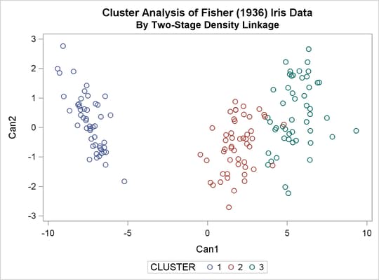
The second analysis uses two-stage density linkage. The raw data suggest two or six modes instead of three:
|
k |
Modes |
|
|---|---|---|
|
3 |
12 |
|
|
4-6 |
6 |
|
|
7 |
4 |
|
|
8 |
3 |
|
|
9-50 |
2 |
|
|
51+ |
1 |
The following analysis uses K=8 to produce three clusters for comparison with other analyses. There are only six misclassifications. The results are shown in Output 33.3.5 and Output 33.3.6.
title2 'By Two-Stage Density Linkage';

proc cluster data=sashelp.iris method=twostage k=8 print=15 ccc pseudo;
   var petal: sepal:;
   copy species;
run;

proc tree noprint ncl=3 out=out;
   copy petal: sepal: species;
run;

%show;
Output 33.3.5: Cluster Analysis of Fisher’s Iris Data: PROC CLUSTER with METHOD=TWOSTAGE
| Cluster Analysis of Fisher (1936) Iris Data |
| By Two-Stage Density Linkage |
| Eigenvalues of the Covariance Matrix | ||||
|---|---|---|---|---|
| Eigenvalue | Difference | Proportion | Cumulative | |
| 1 | 422.824171 | 398.557096 | 0.9246 | 0.9246 |
| 2 | 24.267075 | 16.446125 | 0.0531 | 0.9777 |
| 3 | 7.820950 | 5.437441 | 0.0171 | 0.9948 |
| 4 | 2.383509 | 0.0052 | 1.0000 | |
| Cluster History | |||||||||||||
|---|---|---|---|---|---|---|---|---|---|---|---|---|---|
| Number of Clusters |
Freq | Semipartial R-Square |
R-Square | Approximate Expected R-Square |
Cubic Clustering Criterion |
Pseudo F Statistic |
Pseudo t-Squared |
Normalized Fusion Density |
Maximum Density in Each Cluster |
Tie | |||
| Clusters Joined | Lesser | Greater | |||||||||||
| 15 | CL17 | OB144 | 44 | 0.0025 | .916 | .958 | -11 | 105 | 3.4 | 0.3903 | 0.2066 | 3.5156 | |
| 14 | CL16 | OB44 | 50 | 0.0023 | .913 | .955 | -11 | 110 | 5.6 | 0.3637 | 0.1837 | 100.0 | |
| 13 | CL15 | OB127 | 45 | 0.0029 | .910 | .953 | -10 | 116 | 3.7 | 0.3553 | 0.2130 | 3.5156 | |
| 12 | CL28 | OB66 | 46 | 0.0036 | .907 | .950 | -8.0 | 122 | 5.2 | 0.3223 | 0.1736 | 8.3678 | T |
| 11 | CL12 | OB73 | 47 | 0.0036 | .903 | .946 | -7.6 | 130 | 4.8 | 0.3223 | 0.1736 | 8.3678 | |
| 10 | CL11 | OB79 | 48 | 0.0033 | .900 | .942 | -7.1 | 140 | 4.1 | 0.2879 | 0.1479 | 8.3678 | |
| 9 | CL13 | OB112 | 46 | 0.0037 | .896 | .936 | -6.5 | 152 | 4.4 | 0.2802 | 0.2005 | 3.5156 | |
| 8 | CL10 | OB113 | 49 | 0.0019 | .894 | .930 | -5.5 | 171 | 2.2 | 0.2699 | 0.1372 | 8.3678 | |
| 7 | CL8 | OB91 | 50 | 0.0035 | .891 | .921 | -4.5 | 194 | 4.0 | 0.2586 | 0.1372 | 8.3678 | |
| 6 | CL9 | OB120 | 47 | 0.0042 | .886 | .911 | -3.3 | 225 | 4.6 | 0.1412 | 0.0832 | 3.5156 | |
| 5 | CL6 | OB118 | 48 | 0.0049 | .882 | .895 | -1.7 | 270 | 5.0 | 0.107 | 0.0605 | 3.5156 | |
| 4 | CL5 | OB110 | 49 | 0.0049 | .877 | .872 | 0.35 | 346 | 4.7 | 0.0969 | 0.0541 | 3.5156 | |
| 3 | CL4 | OB135 | 50 | 0.0047 | .872 | .827 | 3.28 | 500 | 4.1 | 0.0715 | 0.0370 | 3.5156 | |
| 2 | CL7 | CL3 | 100 | 0.0993 | .773 | .697 | 3.83 | 503 | 91.9 | 2.6277 | 3.5156 | 8.3678 | |
The CLUSTER procedure is not practical for very large data sets because, with most methods, the CPU time is roughly proportional to the square or cube of the number of observations. The FASTCLUS procedure requires time proportional to the number of observations and can therefore be used with much larger data sets than PROC CLUSTER. If you want to hierarchically cluster a very large data set, you can use PROC FASTCLUS for a preliminary cluster analysis to produce a large number of clusters and then use PROC CLUSTER to hierarchically cluster the preliminary clusters.
FASTCLUS automatically creates the variables _FREQ_ and _RMSSTD_ in the MEAN= output data set. These variables are then automatically used by PROC CLUSTER in the computation of various statistics.
The following SAS code uses the iris data to illustrate the process of clustering clusters. In the preliminary analysis, PROC FASTCLUS produces ten clusters, which are then crosstabulated with species. The data set containing the preliminary clusters is sorted in preparation for later merges. The results are shown in Output 33.3.9 and Output 33.3.10.
title2 'Preliminary Analysis by FASTCLUS';
proc fastclus data=sashelp.iris summary maxc=10 maxiter=99 converge=0
              mean=mean out=prelim cluster=preclus;
   var petal: sepal:;
run;

proc freq;
   tables preclus*species / nopercent norow nocol plot=none;
run;

proc sort data=prelim;
   by preclus;
run;
Output 33.3.9: Preliminary Analysis of Fisher’s Iris Data: FASTCLUS Procedure
| Cluster Summary | ||||||
|---|---|---|---|---|---|---|
| Cluster | Frequency | RMS Std Deviation | Maximum Distance from Seed to Observation |
Radius Exceeded |
Nearest Cluster | Distance Between Cluster Centroids |
| 1 | 14 | 2.3258 | 6.6047 | 10 | 5.6068 | |
| 2 | 16 | 2.0402 | 6.7373 | 3 | 6.2977 | |
| 3 | 23 | 1.6115 | 6.3775 | 8 | 5.4185 | |
| 4 | 24 | 2.4329 | 8.3178 | 6 | 9.3274 | |
| 5 | 10 | 3.1829 | 7.9517 | 4 | 12.4281 | |
| 6 | 18 | 2.2628 | 7.1135 | 7 | 8.2685 | |
| 7 | 12 | 1.9824 | 7.0833 | 1 | 7.6733 | |
| 8 | 11 | 1.7123 | 7.0435 | 3 | 5.4185 | |
| 9 | 10 | 2.5155 | 6.1335 | 10 | 8.4783 | |
| 10 | 12 | 2.0207 | 7.9390 | 1 | 5.6068 | |
Output 33.3.10: Crosstabulation of Species and Cluster From the FASTCLUS Procedure
| Cluster Analysis of Fisher (1936) Iris Data |
| Preliminary Analysis by FASTCLUS |
|
|
|||||||||||||||||||||||||||||||||||||||||||||||||||||||||||||||||||||||||||||||||||||||||||||||||||||||||||||||||||
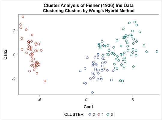
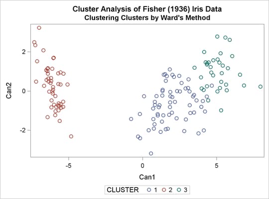
The following macro, CLUS, clusters the preliminary clusters. There is one argument to choose the METHOD= specification to be used by PROC CLUSTER. The TREE procedure creates an output data set containing the three-cluster partition, which is sorted and merged with the OUT= data set from PROC FASTCLUS to determine which cluster each of the original 150 observations belongs to. The SHOW macro is then used to display the results. In this example, the CLUS macro is invoked using Ward’s method, which produces 16 misclassifications, and Wong’s hybrid method, which produces 22 misclassifications.
/*--- Define macro clus ---*/
%macro clus(method);
   proc cluster data=mean method=&method ccc pseudo;
      var petal: sepal:;
      copy preclus;
   run;

   proc tree noprint ncl=3 out=out;
      copy petal: sepal: preclus;
   run;

   proc sort data=out;
      by preclus;
   run;

   data clus;
      merge out prelim;
      by preclus;
   run;

   %show;
%mend;
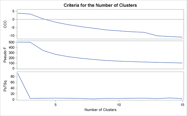
The following statements produce Output 33.3.11 through Output 33.3.14.
title2 'Clustering Clusters by Ward''s Method';
%clus(ward);
Output 33.3.11: Clustering Clusters by Ward’s Method
| Cluster Analysis of Fisher (1936) Iris Data |
| Clustering Clusters by Ward's Method |
| Eigenvalues of the Covariance Matrix | ||||
|---|---|---|---|---|
| Eigenvalue | Difference | Proportion | Cumulative | |
| 1 | 417.301104 | 398.455363 | 0.9504 | 0.9504 |
| 2 | 18.845742 | 16.244505 | 0.0429 | 0.9933 |
| 3 | 2.601236 | 2.272553 | 0.0059 | 0.9993 |
| 4 | 0.328684 | 0.0007 | 1.0000 | |
| Cluster History | ||||||||||
|---|---|---|---|---|---|---|---|---|---|---|
| Number of Clusters |
Clusters Joined | Freq | Semipartial R-Square |
R-Square | Approximate Expected R-Square |
Cubic Clustering Criterion |
Pseudo F Statistic |
Pseudo t-Squared |
Tie | |
| 9 | OB1 | OB10 | 26 | 0.0030 | .957 | .934 | 5.84 | 394 | 10.6 | |
| 8 | OB3 | OB8 | 34 | 0.0032 | .954 | .927 | 6.16 | 420 | 20.2 | |
| 7 | OB6 | OB7 | 30 | 0.0072 | .947 | .919 | 5.70 | 424 | 26.5 | |
| 6 | CL9 | OB9 | 36 | 0.0094 | .937 | .908 | 5.26 | 431 | 24.5 | |
| 5 | OB2 | CL8 | 50 | 0.0103 | .927 | .893 | 5.36 | 461 | 41.3 | |
| 4 | OB4 | OB5 | 34 | 0.0160 | .911 | .870 | 3.84 | 498 | 38.4 | |
| 3 | CL6 | CL7 | 66 | 0.0285 | .883 | .825 | 4.36 | 552 | 48.8 | |
| 2 | CL3 | CL4 | 100 | 0.1099 | .773 | .695 | 3.91 | 503 | 113 | |
| 1 | CL2 | CL5 | 150 | 0.7726 | .000 | .000 | 0.00 | . | 503 | |
The following statements produce Output 33.3.15 through Output 33.3.17.
title2 "Clustering Clusters by Wong's Hybrid Method";
%clus(twostage hybrid);
Output 33.3.15: Clustering Clusters by Wong’s Hybrid Method
| Cluster Analysis of Fisher (1936) Iris Data |
| Clustering Clusters by Wong's Hybrid Method |
| Eigenvalues of the Covariance Matrix | ||||
|---|---|---|---|---|
| Eigenvalue | Difference | Proportion | Cumulative | |
| 1 | 417.301104 | 398.455363 | 0.9504 | 0.9504 |
| 2 | 18.845742 | 16.244505 | 0.0429 | 0.9933 |
| 3 | 2.601236 | 2.272553 | 0.0059 | 0.9993 |
| 4 | 0.328684 | 0.0007 | 1.0000 | |
| Cluster History | |||||||||||||
|---|---|---|---|---|---|---|---|---|---|---|---|---|---|
| Number of Clusters |
Freq | Semipartial R-Square |
R-Square | Approximate Expected R-Square |
Cubic Clustering Criterion |
Pseudo F Statistic |
Pseudo t-Squared |
Normalized Fusion Density |
Maximum Density in Each Cluster |
Tie | |||
| Clusters Joined | Lesser | Greater | |||||||||||
| 9 | OB3 | OB8 | 34 | 0.0032 | .957 | .934 | 5.77 | 392 | 20.2 | 47.595 | 41.5390 | 100.0 | |
| 8 | CL9 | OB2 | 50 | 0.0103 | .947 | .927 | 4.19 | 360 | 41.3 | 34.03 | 28.1852 | 100.0 | |
| 7 | OB1 | OB10 | 26 | 0.0030 | .944 | .919 | 4.94 | 399 | 10.6 | 17.044 | 14.8854 | 22.9763 | |
| 6 | OB6 | OB7 | 30 | 0.0072 | .936 | .908 | 5.07 | 424 | 26.5 | 10.842 | 20.6497 | 24.8051 | |
| 5 | CL6 | OB4 | 54 | 0.0169 | .920 | .893 | 4.00 | 415 | 38.4 | 9.7472 | 20.0098 | 24.8051 | |
| 4 | CL7 | OB9 | 36 | 0.0094 | .910 | .870 | 3.74 | 493 | 24.5 | 7.0911 | 8.2711 | 22.9763 | |
| 3 | CL5 | OB5 | 64 | 0.0347 | .875 | .825 | 3.72 | 517 | 47.7 | 3.4164 | 3.2270 | 24.8051 | |
| 2 | CL3 | CL4 | 100 | 0.1029 | .773 | .695 | 3.91 | 503 | 98.5 | 10.77 | 22.9763 | 24.8051 | |
| 1 | CL2 | CL8 | 150 | 0.7726 | .000 | .000 | 0.00 | . | 503 | 0.5153 | 24.8051 | 100.0 | |