The VARIOGRAM Procedure

The VARIOGRAM procedure computes the empirical (also known as sample or experimental) semivariogram from a set of point measurements. Semivariograms are used in the first steps of spatial prediction as tools that provide insight into the spatial continuity and structure of a random process. Naturally occurring randomness is accounted for by describing a process in terms of the spatial random field (SRF) concept (Christakos, 1992). An SRF is a collection of random variables throughout your spatial domain of prediction. For some of them you already have measurements, and your data set constitutes part of a single realization of this SRF. Based on your sample, spatial prediction aims to provide you with values of the SRF at locations where no measurements are available.

Prediction of the SRF values at unsampled locations by techniques such as ordinary kriging requires the use of a theoretical semivariogram or covariance model. Due to the randomness involved in stochastic processes, the theoretical semivariance cannot be computed. Instead, it is possible that the empirical semivariance can provide an estimate of the theoretical semivariance, which then characterizes the spatial structure of the process.

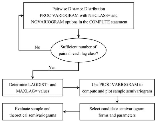
The VARIOGRAM procedure follows a general flow of investigation that leads you from a set of spatial observations to an expression of theoretical semivariance to characterize the SRF continuity. Specifically, the empirical semivariogram is computed after a suitable choice is made for the LAGDISTANCE= and MAXLAGS= options. For computations in more than one direction you can further use the NDIRECTIONS= option or the DIRECTIONS statement. Potential theoretical models (which can also incorporate nesting, anisotropy, and the nugget effect) can be fitted to the empirical semivariance by using the MODEL statement, and then plotted against the empirical semivariogram. The flow of this analytical process is illustrated in Figure 106.17. After a suitable theoretical model is determined, it is used in PROC KRIGE2D for the prediction stage. The prediction analysis is presented in detail in the section Details of Ordinary Kriging in Chapter 53: The KRIGE2D Procedure.

It is critical to note that the empirical semivariance provides an estimate of its theoretical counterpart only when the SRF satisfies stationarity conditions. These conditions imply that the SRF has a constant (or zero) expected value. Consequently, your data need to be sampled from a trend-free random field and need to have a constant mean, as assumed in Getting Started: VARIOGRAM Procedure. Equivalently, your data could be residuals of an initial sample that has had a surface trend removed, as portrayed in An Anisotropic Case Study with Surface Trend in the Data. For a closer look at stationarity, see the section Stationarity. For details about different stationarity types and conditions see, for example, Chilès and Delfiner (1999, section 1.1.4).