The SURVEYMEANS Procedure

Let Y be the variable of interest in a complex survey. Denote ![]() as the cumulative distribution function of Y. For
as the cumulative distribution function of Y. For ![]() , the pth quantile of the population cumulative distribution function is
, the pth quantile of the population cumulative distribution function is
Let ![]() be the observed values for variable Y that are associated with sampling weights, where
be the observed values for variable Y that are associated with sampling weights, where ![]() are the stratum index, cluster index, and member index, respectively, as shown in the section Definitions and Notation. Let
are the stratum index, cluster index, and member index, respectively, as shown in the section Definitions and Notation. Let ![]() denote the sample order statistics for variable Y.
denote the sample order statistics for variable Y.
An estimate of quantile ![]() is
is
![\[ \hat Q(p)= \left\{ \begin{array}{ll} y_{(1)} & \mbox{ if } p<\hat F(y_{(1)}) \\ y_{(k)}+\displaystyle {\frac{p-\hat F(y_{(k)})}{\hat F(y_{(k+1)})-\hat F(y_{(k)})}} (y_{(k+1)}-y_{(k)}) & \mbox{ if } \hat F(y_{(k)}) \le p < \hat F(y_{(k+1)}) \\ y_{(n)} & \mbox{ if } p=1 \end{array} \right. \]](images/statug_surveymeans0110.png)
where ![]() is the estimated cumulative distribution for Y,
is the estimated cumulative distribution for Y,
and ![]() is the indicator function.
is the indicator function.
When you specify VARMETHOD=TAYLOR, or by default if you do not specify the VARMETHOD= option, PROC SURVEYMEANS uses Woodruff’s method (Dorfman and Valliant, 1993; Särndal, Swensson, and Wretman, 1992; Francisco and Fuller, 1991) to estimate the variances of quantiles. This method first constructs a confidence interval on a quantile. Then it uses the width of the confidence interval to estimate the standard error of a quantile.
In order to estimate the variance of ![]() , PROC SURVEYMEANS first estimates the variance of the estimated distribution function
, PROC SURVEYMEANS first estimates the variance of the estimated distribution function ![]() by
by
where
Then ![]() % confidence limits for
% confidence limits for ![]() can be constructed by
can be constructed by
where ![]() is the
is the ![]() percentile of the t distribution with df degrees of freedom, described in the section Degrees of Freedom.
percentile of the t distribution with df degrees of freedom, described in the section Degrees of Freedom.
When ![]() is out of the range of [0,1], the procedure does not compute the standard error of
is out of the range of [0,1], the procedure does not compute the standard error of ![]() .
.
The ![]() th quantile is defined as
th quantile is defined as
![\[ \hat Q(\hat p_ L)= \left\{ \begin{array}{ll} y_{(1)} & \mbox{ if } \hat p_ L<\hat F(y_{(1)}) \\ y_{(k_ L)}+\displaystyle {\frac{\hat p_ L-\hat F(y_{(k_ L)})}{\hat F(y_{(k_ L+1)})-\hat F(y_{(k_ L)})}} (y_{(k_ L+1)}-y_{(k_ L)}) & \mbox{ if } \hat F(y_{(k_ L)}) \le \hat p_ L < \hat F(y_{(k_ L+1)}) \\ y_{(d)} & \mbox{ if } \hat p_ L=1 \end{array} \right. \]](images/statug_surveymeans0121.png)
and the ![]() th quantile is defined as
th quantile is defined as
![\[ \hat Q(\hat p_ U)= \left\{ \begin{array}{ll} y_{(1)} & \mbox{ if } \hat p_ U<\hat F(y_{(1)}) \\ y_{(k_ U)}+\displaystyle {\frac{\hat p_ U-\hat F(y_{(k_ U)})}{\hat F(y_{(k_ U+1)})-\hat F(y_{(k_ U)})}} (y_{(k_ U+1)}-y_{(k_ U)}) & \mbox{ if } \hat F(y_{(k_ U)}) \le \hat p_ U < \hat F(y_{(k_ U+1)}) \\ y_{(d)} & \mbox{ if } \hat p_ U=1 \end{array} \right. \]](images/statug_surveymeans0123.png)
The standard error of ![]() is then estimated by
is then estimated by
where ![]() is the
is the ![]() percentile of the t distribution with df degrees of freedom.
percentile of the t distribution with df degrees of freedom.
When you use the replication method, PROC SURVEYMEANS uses the usual variance estimates for a quantile as described in the section Replication Methods for Variance Estimation. However, you should proceed cautiously, because this variance estimator can have poor properties (Dorfman and Valliant, 1993).
Symmetric ![]() % confidence limits are computed as
% confidence limits are computed as
If you specify the NONSYMCL option in the PROC SURVEYMEANS statement when you use the VARMETHOD=TAYLOR option, the procedure computes ![]() % nonsymmetric confidence limits:
% nonsymmetric confidence limits:
When you specify a POSTSTRATA statement, the quantile estimation and its variance estimation incorporate poststratification. For more information about poststratification, see the section Poststratification.
For a selected sample, let ![]() be the poststratum index; let
be the poststratum index; let ![]() be the population totals for each corresponding poststratum, and let
be the population totals for each corresponding poststratum, and let ![]() be the indicator variable for the poststratum r that is defined by
be the indicator variable for the poststratum r that is defined by
Denote the total sum of original weights in the sample for each poststratum as
Assume that the observation (h, i, j) belongs to the rth poststratum. Then the poststratification weight for the observation (h, i, j) is
Then the estimated cumulative distribution function of Y, ![]() and the estimated pth quantile estimation
and the estimated pth quantile estimation ![]() can be computed as in the section Estimate of Quantile by replacing the original weights,
can be computed as in the section Estimate of Quantile by replacing the original weights, ![]() , with the poststratification weights,
, with the poststratification weights, ![]() .
.
When you specify VARMETHOD=TAYLOR (or by default), the variance of ![]() is estimated as in the section Standard Error, except that the variance of the estimated distribution function
is estimated as in the section Standard Error, except that the variance of the estimated distribution function ![]() is computed as follows.
is computed as follows.
For each poststratum ![]() , define
, define
where ![]() is the indicator function.
is the indicator function.
Assume that the observation (h, i, j) belongs to the rth poststratum. Let
PROC SURVEYMEANS estimates the variance of the estimated distribution function ![]() with poststratification by
with poststratification by
where
Let Y be the variable of interest in a complex survey, and let a subpopulation of interest be domain D. Denote ![]() as the cumulative distribution function of Y in domain D. For
as the cumulative distribution function of Y in domain D. For ![]() , the pth quantile of the population cumulative distribution function is
, the pth quantile of the population cumulative distribution function is
Let ![]() be the corresponding indicator variable:
be the corresponding indicator variable:
Assume that there are a total of d observations among the n observations in the entire sample that belong to domain D. Let ![]() denote the order statistics of variable Y for these d observations that fall in domain D.
denote the order statistics of variable Y for these d observations that fall in domain D.
The cumulative distribution function of Y in domain D is estimated by
and ![]() is the indicator function. Then the estimated quantile in domain D is
is the indicator function. Then the estimated quantile in domain D is
![\[ \hat Q_ D(p)= \left\{ \begin{array}{ll} y_{(1)} & \mbox{ if } p<\hat F_ D(y_{(1)}) \\ y_{(k)}+\displaystyle {\frac{p-\hat F_ D(y_{(k)})}{\hat F_ D(y_{(k+1)})-\hat F_ D(y_{(k)})}} (y_{(k+1)}-y_{(k)}) & \mbox{ if } \hat F_ D(y_{(k)}) \le p < \hat F_ D(y_{(k+1)}) \\ y_{(d)} & \mbox{ if } p=1 \end{array} \right. \]](images/statug_surveymeans0143.png)
In order to estimate the variance for ![]() , PROC SURVEYMEANS first estimates the variance of the estimated distribution function
, PROC SURVEYMEANS first estimates the variance of the estimated distribution function ![]() in domain D. When you specify VARMETHOD=TAYLOR (or by default), the variance of
in domain D. When you specify VARMETHOD=TAYLOR (or by default), the variance of ![]() is estimated by
is estimated by
where
Then ![]() % confidence limits for
% confidence limits for ![]() can be constructed by
can be constructed by ![]() , where
, where
and ![]() is the
is the ![]() percentile of the t distribution with df degrees of freedom, described in the section Degrees of Freedom. When
percentile of the t distribution with df degrees of freedom, described in the section Degrees of Freedom. When ![]() is out of the range of [0,1], PROC SURVEYMEANS does not compute the standard error of
is out of the range of [0,1], PROC SURVEYMEANS does not compute the standard error of ![]() .
.
The ![]() th quantile is then estimated as
th quantile is then estimated as
![\[ \hat Q_ D(\hat{p}_{DL})= \left\{ \begin{array}{ll} y_{(1)} & \mbox{ if } \hat{p}_{DL}<\hat F_ D(y_{(1)}) \\ y_{(k_ L)}+\displaystyle {\frac{(\hat{p}_{DL}-\hat F_ D(y_{(k_ L)}))(y_{(k_ L+1)}-y_{(k_ L)})}{\hat F_ D(y_{(k_ L+1)})-\hat F_ D(y_{(k_ L)})}} & \mbox{ if } \hat F_ D(y_{(k_ L)}) \le \hat p_{DL} < \hat F_ D(y_{(k_ L+1)}) \\ y_{(d)} & \mbox{ if } \hat p_{DL}=1 \end{array} \right. \]](images/statug_surveymeans0151.png)
The ![]() th quantile is then estimated as
th quantile is then estimated as
![\[ \hat Q_ D(\hat{p}_{DU})= \left\{ \begin{array}{ll} y_{(1)} & \mbox{ if } \hat{p}_{DU}<\hat F_ D(y_{(1)}) \\ y_{(k_ U)}+\displaystyle {\frac{(\hat{p}_{DU}-\hat F_ D(y_{(k_ U)}))(y_{(k_ U+1)}-y_{(k_ U)})}{\hat F_ D(y_{(k_ U+1)})-\hat F_ D(y_{(k_ U)})}} & \mbox{ if } \hat F_ D(y_{(k_ U)}) \le \hat p_{DU} < \hat F_ D(y_{(k_ U+1)}) \\ y_{(d)} & \mbox{ if } \hat p_{DU}=1 \end{array} \right. \]](images/statug_surveymeans0153.png)
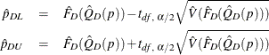
The standard error of ![]() is then estimated by
is then estimated by
where ![]() is the
is the ![]() percentile of the t distribution with df degrees of freedom.
percentile of the t distribution with df degrees of freedom.
Symmetric ![]() % confidence limits for
% confidence limits for ![]() are computed as
are computed as
If you specify the NONSYMCL option in the PROC SURVEYMEANS statement, the procedure displays ![]() % nonsymmetric confidence limits as
% nonsymmetric confidence limits as
When you specify both a POSTSTRATA statement and a DOMAIN statement, the domain quantile estimation and its variance estimation incorporate poststratification. For more information about poststratification, see the section Poststratification.
For a selected sample, let ![]() be the poststratum index, let
be the poststratum index, let ![]() be the population totals for each corresponding poststratum, and let
be the population totals for each corresponding poststratum, and let ![]() be the indicator variable for the poststratum r:
be the indicator variable for the poststratum r:
The poststratification weights, ![]() , are defined as in the section Quantile Estimation with Poststratification.
, are defined as in the section Quantile Estimation with Poststratification.
For domain D, let ![]() be the corresponding indicator variable:
be the corresponding indicator variable:
With poststratification, for variable Y, the estimated cumulative distribution in domain D, ![]() , and its pth quantile estimation,
, and its pth quantile estimation, ![]() , can be computed as in the section Domain Quantile by replacing the original weights,
, can be computed as in the section Domain Quantile by replacing the original weights, ![]() , with the poststratification weights,
, with the poststratification weights, ![]() . However, the variance of
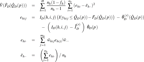
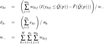
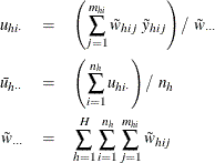
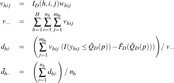
. However, the variance of ![]() , which is described in the section Domain Quantile, is computed as follows when you specify the VARMETHOD=TAYLOR option (or by default).
, which is described in the section Domain Quantile, is computed as follows when you specify the VARMETHOD=TAYLOR option (or by default).
Define
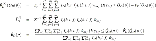
Assume that the observation (h, i, j) belongs to the rth poststratum. Then the variance of ![]() is estimated by
is estimated by