The SIMNORMAL Procedure

The following example illustrates the use of PROC SIMNORMAL to generate variable values conditioned on a set of related or correlated variables.
Suppose you are given a sample of size 50 from ten normally distributed, correlated random variables, ![]() . The first five variables represent input variables for a chemical manufacturing process, and the last five are output variables.
. The first five variables represent input variables for a chemical manufacturing process, and the last five are output variables.
First, the data are input and the correlation structure is determined by using PROC CORR, as in the following statements. The results are shown in Figure 90.2.
data a ;
   input in1-in5 out1-out5 ;
   datalines ;
 9.3500    10.0964     7.3177    10.3617    10.3444    9.4612
10.7443     9.9026     9.0144    11.7968
 7.8599    10.4560    10.0075     8.5875    10.0014   10.3869

   ... more lines ...

 8.9174     9.9623     9.5742     9.9713
run ;
proc corr data=a cov nocorr outp=outcov ;
   var in1-in5 out1-out5 ;
run ;
Figure 90.2: Correlation of Chemical Process Variables
| Statistics for PROC SIMNORM Sample Using NUMREAL=5000 |
| 10 Variables: | in1 in2 in3 in4 in5 out1 out2 out3 out4 out5 |
|---|
| Covariance Matrix, DF = 49 | ||||||||||
|---|---|---|---|---|---|---|---|---|---|---|
| in1 | in2 | in3 | in4 | in5 | out1 | out2 | out3 | out4 | out5 | |
| in1 | 1.019198331 | 0.128086799 | 0.291646382 | 0.327014916 | 0.417546732 | 0.097650713 | 0.206698403 | 0.516271121 | 0.118726106 | 0.261770905 |
| in2 | 0.128086799 | 1.056460818 | 0.143581799 | 0.095937707 | 0.104117743 | 0.056612934 | -0.121700731 | 0.266581451 | 0.092288067 | -0.020971411 |
| in3 | 0.291646382 | 0.143581799 | 1.384051249 | 0.058853960 | 0.326107730 | 0.093498839 | 0.078294087 | 0.481576554 | 0.057816322 | 0.259053423 |
| in4 | 0.327014916 | 0.095937707 | 0.058853960 | 1.023128678 | 0.347916864 | 0.022915645 | 0.125961491 | 0.179627237 | 0.075028230 | 0.078147576 |
| in5 | 0.417546732 | 0.104117743 | 0.326107730 | 0.347916864 | 1.606858140 | 0.360270318 | 0.297046593 | 0.749212945 | 0.220196337 | 0.349618466 |
| out1 | 0.097650713 | 0.056612934 | 0.093498839 | 0.022915645 | 0.360270318 | 0.807007554 | 0.217285879 | 0.064816340 | -0.053931448 | 0.037758721 |
| out2 | 0.206698403 | -0.121700731 | 0.078294087 | 0.125961491 | 0.297046593 | 0.217285879 | 0.929455806 | 0.206825664 | 0.138551008 | 0.054039499 |
| out3 | 0.516271121 | 0.266581451 | 0.481576554 | 0.179627237 | 0.749212945 | 0.064816340 | 0.206825664 | 1.837505268 | 0.292963975 | 0.165910481 |
| out4 | 0.118726106 | 0.092288067 | 0.057816322 | 0.075028230 | 0.220196337 | -0.053931448 | 0.138551008 | 0.292963975 | 0.832831377 | -0.067396486 |
| out5 | 0.261770905 | -0.020971411 | 0.259053423 | 0.078147576 | 0.349618466 | 0.037758721 | 0.054039499 | 0.165910481 | -0.067396486 | 0.697717191 |
| Simple Statistics | ||||||
|---|---|---|---|---|---|---|
| Variable | N | Mean | Std Dev | Sum | Minimum | Maximum |
| in1 | 50 | 10.18988 | 1.00955 | 509.49400 | 7.63500 | 12.58860 |
| in2 | 50 | 10.10673 | 1.02784 | 505.33640 | 8.12580 | 13.78310 |
| in3 | 50 | 10.14888 | 1.17646 | 507.44420 | 7.31770 | 12.40080 |
| in4 | 50 | 10.03884 | 1.01150 | 501.94200 | 7.40490 | 11.99060 |
| in5 | 50 | 10.22587 | 1.26762 | 511.29340 | 7.23350 | 12.93360 |
| out1 | 50 | 9.85347 | 0.89834 | 492.67340 | 8.01220 | 12.24660 |
| out2 | 50 | 9.96857 | 0.96408 | 498.42840 | 7.76420 | 12.09450 |
| out3 | 50 | 10.29588 | 1.35555 | 514.79410 | 7.29660 | 13.74200 |
| out4 | 50 | 10.15856 | 0.91260 | 507.92780 | 8.43090 | 12.45230 |
| out5 | 50 | 10.26023 | 0.83529 | 513.01130 | 7.86060 | 11.96000 |
After the mean and correlation structure are determined, any subset of these variables can be simulated. Suppose you are interested in a particular function of the output variables for two sets of values of the input variables for the process. In particular, you are interested in the mean and variability of the following function over 500 runs of the process conditioned on each set of input values:
Although the distribution of these quantities could be determined theoretically, it is simpler to perform a conditional simulation by using PROC SIMNORMAL.
To do this, you first append a _TYPE_=’COND’ observation to the covariance data set produced by PROC CORR for each group of input values:
data cond1 ;
   _TYPE_='COND' ;
   in1 = 8    ;
   in2 = 10.5 ;
   in3 = 12   ;
   in4 = 13.5 ;
   in5 = 14.4 ;
   output ;
run ;

data cond2 ;
   _TYPE_='COND' ;
   in1 = 15.4 ;
   in2 = 13.7 ;
   in3 = 11 ;
   in4 = 7.9 ;
   in5 = 5.5 ;
   output ;
run ;
Next, each of these conditioning observations is appended to a copy of the OUTP=OUTCOV data from the CORR procedure, as in
the following statements. A new variable, INPUT, is added to distinguish the sets of input values. This variable is used as a BY variable in subsequent steps.
data outcov1 ;
   input=1 ;
   set outcov cond1 ;
run ;

data outcov2 ;
   input=2 ;
   set outcov cond2 ;
run ;
Finally, these two data sets are concatenated:
data outcov ;
   set outcov1 outcov2 ;
run ;
proc print data=outcov ;
   where (_type_ ne 'COV') ;
run ;
Figure 90.3 shows the added observations.
Figure 90.3: OUTP= Data Set from PROC CORR with _TYPE_=COND Observations Appended
| Statistics for PROC SIMNORM Sample Using NUMREAL=5000 |
| Obs | input | _TYPE_ | _NAME_ | in1 | in2 | in3 | in4 | in5 | out1 | out2 | out3 | out4 | out5 |
|---|---|---|---|---|---|---|---|---|---|---|---|---|---|
| 11 | 1 | MEAN | 10.1899 | 10.1067 | 10.1489 | 10.0388 | 10.2259 | 9.8535 | 9.9686 | 10.2959 | 10.1586 | 10.2602 | |
| 12 | 1 | STD | 1.0096 | 1.0278 | 1.1765 | 1.0115 | 1.2676 | 0.8983 | 0.9641 | 1.3555 | 0.9126 | 0.8353 | |
| 13 | 1 | N | 50.0000 | 50.0000 | 50.0000 | 50.0000 | 50.0000 | 50.0000 | 50.0000 | 50.0000 | 50.0000 | 50.0000 | |
| 14 | 1 | COND | 8.0000 | 10.5000 | 12.0000 | 13.5000 | 14.4000 | . | . | . | . | . | |
| 25 | 2 | MEAN | 10.1899 | 10.1067 | 10.1489 | 10.0388 | 10.2259 | 9.8535 | 9.9686 | 10.2959 | 10.1586 | 10.2602 | |
| 26 | 2 | STD | 1.0096 | 1.0278 | 1.1765 | 1.0115 | 1.2676 | 0.8983 | 0.9641 | 1.3555 | 0.9126 | 0.8353 | |
| 27 | 2 | N | 50.0000 | 50.0000 | 50.0000 | 50.0000 | 50.0000 | 50.0000 | 50.0000 | 50.0000 | 50.0000 | 50.0000 | |
| 28 | 2 | COND | 15.4000 | 13.7000 | 11.0000 | 7.9000 | 5.5000 | . | . | . | . | . |
You now run PROC SIMNORMAL, specifying the input data set and the VAR and COND variables. Note that you must specify a TYPE=COV
or TYPE=CORR for the input data set. PROC CORR automatically assigns a TYPE=COV or TYPE=CORR attribute for the OUTP= data
set. However, since the intermediate DATA steps that appended the _TYPE_=’COND’ observations turned off this attribute, an
explicit TYPE=CORR in the DATA= option in the PROC SIMNORMAL statement is needed.
The specification of PROC SIMNORMAL now follows from the problem description. The condition variables are IN1–IN5, the analysis
variables are OUT1–OUT5, and 500 realizations are required. A seed value can be chosen arbitrarily, or the system clock can
be used. Note that in the following statements, the simulation is done for each of the values of the BY variable INPUT:
proc simnormal data=outcov(type=cov)
      out = osim
      numreal = 500
      seed = 33179
      ;
   by input ;
   var out1-out5 ;
   cond in1-in5 ;
run;

data b;
   set osim ;
   denom = sum(of out1-out5) ;
   if abs(denom) < 1e-8 then ff = . ;
   else ff = (out1-out3)/denom ;
run ;
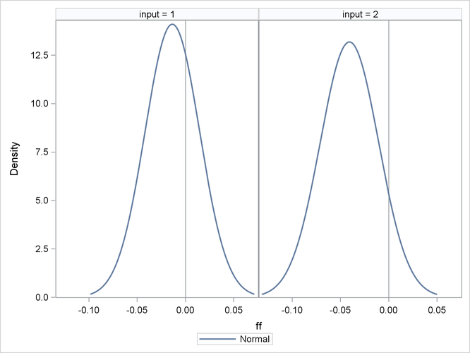
The DATA step that follows the simulation computes the function ![]() ; in the following statements the UNIVARIATE procedure computes the simple statistics for this function for each set of conditioning
input values. This is shown in Figure 90.4, and Figure 90.5 shows the distribution of the function values for each set of input values by using the SGPANEL procedure.
; in the following statements the UNIVARIATE procedure computes the simple statistics for this function for each set of conditioning
input values. This is shown in Figure 90.4, and Figure 90.5 shows the distribution of the function values for each set of input values by using the SGPANEL procedure.
proc univariate data=b ;
   by input ;
   var ff ;
run ;
title ;
proc sgpanel data=b ;
   panelby input ;
   REFLINE 0 / axis= x ;
   density ff ;
run ;
Figure 90.4: Simple Statistics for ff for Each Set of Input Values
| Statistics for PROC SIMNORM Sample Using NUMREAL=5000 |
| Moments | |||
|---|---|---|---|
| N | 500 | Sum Weights | 500 |
| Mean | -0.0134833 | Sum Observations | -6.7416303 |
| Std Deviation | 0.02830426 | Variance | 0.00080113 |
| Skewness | 0.56773239 | Kurtosis | 1.31522925 |
| Uncorrected SS | 0.49066351 | Corrected SS | 0.39976435 |
| Coeff Variation | -209.92145 | Std Error Mean | 0.0012658 |
| Basic Statistical Measures | |||
|---|---|---|---|
| Location | Variability | ||
| Mean | -0.01348 | Std Deviation | 0.02830 |
| Median | -0.01565 | Variance | 0.0008011 |
| Mode | . | Range | 0.21127 |
| Interquartile Range | 0.03618 | ||
| Tests for Location: Mu0=0 | ||||
|---|---|---|---|---|
| Test | Statistic | p Value | ||
| Student's t | t | -10.6519 | Pr > |t| | <.0001 |
| Sign | M | -106 | Pr >= |M| | <.0001 |
| Signed Rank | S | -33682 | Pr >= |S| | <.0001 |
| Quantiles (Definition 5) | |
|---|---|
| Level | Quantile |
| 100% Max | 0.11268600 |
| 99% | 0.07245656 |
| 95% | 0.03270269 |
| 90% | 0.02064338 |
| 75% Q3 | 0.00370322 |
| 50% Median | -0.01564850 |
| 25% Q1 | -0.03247389 |
| 10% | -0.04716239 |
| 5% | -0.05572806 |
| 1% | -0.07201126 |
| 0% Min | -0.09858350 |
| Extreme Observations | |||
|---|---|---|---|
| Lowest | Highest | ||
| Value | Obs | Value | Obs |
| -0.0985835 | 471 | 0.0750538 | 22 |
| -0.0908179 | 472 | 0.0794747 | 245 |
| -0.0802423 | 90 | 0.0840160 | 48 |
| -0.0760645 | 249 | 0.1004812 | 222 |
| -0.0756070 | 226 | 0.1126860 | 50 |
| Statistics for PROC SIMNORM Sample Using NUMREAL=5000 |
| Moments | |||
|---|---|---|---|
| N | 500 | Sum Weights | 500 |
| Mean | -0.0405913 | Sum Observations | -20.295631 |
| Std Deviation | 0.03027008 | Variance | 0.00091628 |
| Skewness | 0.1033062 | Kurtosis | -0.1458848 |
| Uncorrected SS | 1.28104777 | Corrected SS | 0.4572225 |
| Coeff Variation | -74.57289 | Std Error Mean | 0.00135372 |
| Basic Statistical Measures | |||
|---|---|---|---|
| Location | Variability | ||
| Mean | -0.04059 | Std Deviation | 0.03027 |
| Median | -0.04169 | Variance | 0.0009163 |
| Mode | . | Range | 0.18332 |
| Interquartile Range | 0.04339 | ||
| Tests for Location: Mu0=0 | ||||
|---|---|---|---|---|
| Test | Statistic | p Value | ||
| Student's t | t | -29.985 | Pr > |t| | <.0001 |
| Sign | M | -203 | Pr >= |M| | <.0001 |
| Signed Rank | S | -58745 | Pr >= |S| | <.0001 |
| Quantiles (Definition 5) | |
|---|---|
| Level | Quantile |
| 100% Max | 0.06101208 |
| 99% | 0.02693796 |
| 95% | 0.01008202 |
| 90% | -0.00111776 |
| 75% Q3 | -0.01847726 |
| 50% Median | -0.04169199 |
| 25% Q1 | -0.06187039 |
| 10% | -0.07798499 |
| 5% | -0.08606522 |
| 1% | -0.11026564 |
| 0% Min | -0.12231183 |
| Extreme Observations | |||
|---|---|---|---|
| Lowest | Highest | ||
| Value | Obs | Value | Obs |
| -0.122312 | 937 | 0.0272906 | 688 |
| -0.119884 | 980 | 0.0291769 | 652 |
| -0.113512 | 920 | 0.0388217 | 670 |
| -0.112345 | 523 | 0.0477261 | 845 |
| -0.110497 | 897 | 0.0610121 | 632 |