The POWER Procedure
- Overview
-
Getting Started

-
Syntax
-
Details
-
ExamplesOne-Way ANOVAThe Sawtooth Power Function in Proportion AnalysesSimple AB/BA Crossover DesignsNoninferiority Test with Lognormal DataMultiple Regression and CorrelationComparing Two Survival CurvesConfidence Interval PrecisionCustomizing PlotsBinary Logistic Regression with Independent PredictorsWilcoxon-Mann-Whitney Test
- References
Notation:
|
Outcome |
||||
|
Failure |
Success |
|||
|
Group |
1 |
|
|
|
|
2 |
|
|
|
|
|
|
m |
N |
||
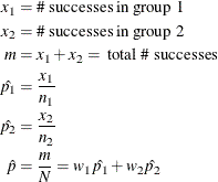
The hypotheses are
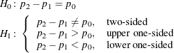
where ![]() is constrained to be 0 for all but the unconditional Pearson chi-square test.
is constrained to be 0 for all but the unconditional Pearson chi-square test.
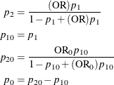
Internal calculations are performed in terms of ![]() ,
, ![]() , and
, and ![]() . An input set consisting of OR,
. An input set consisting of OR, ![]() , and
, and ![]() is transformed as follows:
is transformed as follows:
An input set consisting of RR, ![]() , and
, and ![]() is transformed as follows:
is transformed as follows:

Note that the transformation of either ![]() or
or ![]() to
to ![]() is not unique. The chosen parameterization fixes the null value
is not unique. The chosen parameterization fixes the null value ![]() at the input value of
at the input value of ![]() .
.
The usual Pearson chi-square test is unconditional. The test statistic
![\[ z_ P = \frac{\hat{p_2} - \hat{p_1} - p_0}{\left[ \hat{p}(1-\hat{p}) \left( \frac{1}{n_1} + \frac{1}{n_2} \right) \right]^\frac {1}{2}} \, = \, \left[ N w_1 w_2 \right]^\frac {1}{2} \frac{\hat{p_2} - \hat{p_1} - p_0}{\hat{p}(1-\hat{p})} \]](images/statug_power0422.png)
is assumed to have a null distribution of ![]() .
.
Sample size for the one-sided cases is given by equation (4) in Fleiss, Tytun, and Ury (1980). One-sided power is computed as suggested by Diegert and Diegert (1981) by inverting the sample size formula. Power for the two-sided case is computed by adding the lower-sided and upper-sided
powers each with ![]() , and sample size for the two-sided case is obtained by numerically inverting the power formula. A custom null value
, and sample size for the two-sided case is obtained by numerically inverting the power formula. A custom null value ![]() for the proportion difference
for the proportion difference ![]() is also supported.
is also supported.
![\[ \mr {power} = \left\{ \begin{array}{ll} \Phi \left( \frac{(p_2 - p_1 - p_0) (N w_1 w_2)^\frac {1}{2} - z_{1-\alpha } \left[ (w_1 p_1 + w_2 p_2) (1 - w_1 p_1 - w_2 p_2) \right]^\frac {1}{2}}{\left[ w_2 p_1 (1 - p_1) + w_1 p_2 (1 - p_2) \right]^\frac {1}{2}} \right), & \mbox{upper one-sided} \\ \Phi \left( \frac{-(p_2 - p_1 - p_0) (N w_1 w_2)^\frac {1}{2} - z_{1-\alpha } \left[ (w_1 p_1 + w_2 p_2) (1 - w_1 p_1 - w_2 p_2) \right]^\frac {1}{2}}{\left[ w_2 p_1 (1 - p_1) + w_1 p_2 (1 - p_2) \right]^\frac {1}{2}} \right), & \mbox{lower one-sided} \\ \Phi \left( \frac{(p_2 - p_1 - p_0) (N w_1 w_2)^\frac {1}{2} - z_{1-\frac{\alpha }{2}} \left[ (w_1 p_1 + w_2 p_2) (1 - w_1 p_1 - w_2 p_2) \right]^\frac {1}{2}}{\left[ w_2 p_1 (1 - p_1) + w_1 p_2 (1 - p_2) \right]^\frac {1}{2}} \right) + \\ \quad \Phi \left( \frac{-(p_2 - p_1 - p_0) (N w_1 w_2)^\frac {1}{2} - z_{1-\frac{\alpha }{2}} \left[ (w_1 p_1 + w_2 p_2) (1 - w_1 p_1 - w_2 p_2) \right]^\frac {1}{2}}{\left[ w_2 p_1 (1 - p_1) + w_1 p_2 (1 - p_2) \right]^\frac {1}{2}} \right), & \mbox{two-sided} \\ \end{array} \right. \]](images/statug_power0424.png)
For the one-sided cases, a closed-form inversion of the power equation yield an approximate total sample size
![\[ N = \frac{ \left[ z_{1-\alpha } \left\{ (w_1 p_1 + w_2 p_2) (1 - w_1 p_1 - w_2 p_2) \right\} ^\frac {1}{2} + z_{\mr {power}} \left\{ w_2 p_1 (1 - p_1) + w_1 p_2 (1 - p_2) \right\} ^\frac {1}{2} \right]^2 }{ w_1 w_2 (p_2 - p_1 - p_0)^2 } \]](images/statug_power0425.png)
For the two-sided case, the solution for N is obtained by numerically inverting the power equation.
The usual likelihood ratio chi-square test is unconditional. The test statistic
![\[ z_{\mr {LR}} = (-1_{\{ p_2 < p_1\} })\sqrt {2N \sum _{i=1}^2 \left[ w_ i \hat{p_ i} \log \left( \frac{\hat{p_ i}}{\hat{p}} \right) + w_ i (1-\hat{p_ i}) \log \left( \frac{1-\hat{p_ i}}{1-\hat{p}} \right) \right]} \]](images/statug_power0426.png)
is assumed to have a null distribution of ![]() and an alternative distribution of
and an alternative distribution of ![]() , where
, where
![\[ \delta = N^\frac {1}{2} (-1_{\{ p_2 < p_1\} })\sqrt {2 \sum _{i=1}^2 \left[ w_ i p_ i \log \left( \frac{p_ i}{w_1 p_1 + w_2 p_2} \right) + w_ i (1-p_ i) \log \left( \frac{1-p_ i}{1-(w_1 p_1 + w_2 p_2)} \right) \right]} \]](images/statug_power0428.png)
The approximate power is
![\[ \mr {power} = \left\{ \begin{array}{ll} \Phi \left( \delta - z_{1-\alpha } \right), & \mbox{upper one-sided} \\ \Phi \left( - \delta - z_{1-\alpha } \right), & \mbox{lower one-sided} \\ \Phi \left( \delta - z_{1-\frac{\alpha }{2}} \right) + \Phi \left( - \delta - z_{1-\frac{\alpha }{2}} \right), & \mbox{two-sided} \\ \end{array} \right. \\ \]](images/statug_power0429.png)
For the one-sided cases, a closed-form inversion of the power equation yield an approximate total sample size
For the two-sided case, the solution for N is obtained by numerically inverting the power equation.
Fisher’s exact test is conditional on the observed total number of successes m. Power and sample size computations are based on a test with similar power properties, the continuity-adjusted arcsine test. The test statistic
![\begin{align*} z_ A & = (4N w_1 w_2)^\frac {1}{2} \left[ \mr {arcsin}\left( \left[ \hat{p_2} + \frac{1}{2N w_2} (1_{\{ \hat{p_2} < \hat{p_1}\} } - 1_{\{ \hat{p_2} > \hat{p_1}\} }) \right]^\frac {1}{2} \right) \right. \\ & \quad \left. - \mr {arcsin}\left( \left[ \hat{p_1} + \frac{1}{2N w_1} (1_{\{ \hat{p_1} < \hat{p_2}\} } - 1_{\{ \hat{p_1} > \hat{p_2}\} }) \right]^\frac {1}{2} \right) \right] \end{align*}](images/statug_power0431.png)
is assumed to have a null distribution of ![]() and an alternative distribution of
and an alternative distribution of ![]() , where
, where
![\begin{align*} \delta & = (4N w_1 w_2)^\frac {1}{2} \left[ \mr {arcsin}\left( \left[ p_2 + \frac{1}{2N w_2} (1_{\{ p_2 < p_1\} } - 1_{\{ p_2 > p_1\} }) \right]^\frac {1}{2} \right) \right. \\ & \quad \left. - \mr {arcsin}\left( \left[ p_1 + \frac{1}{2N w_1} (1_{\{ p_1 < p_2\} } - 1_{\{ p_1 > p_2\} }) \right]^\frac {1}{2} \right) \right] \end{align*}](images/statug_power0432.png)
The approximate power for the one-sided balanced case is given by Walters (1979) and is easily extended to the unbalanced and two-sided cases:
The approximation is valid only for ![]() .
.