The POWER Procedure
- Overview
-
Getting Started

-
Syntax
-
Details
-
ExamplesOne-Way ANOVAThe Sawtooth Power Function in Proportion AnalysesSimple AB/BA Crossover DesignsNoninferiority Test with Lognormal DataMultiple Regression and CorrelationComparing Two Survival CurvesConfidence Interval PrecisionCustomizing PlotsBinary Logistic Regression with Independent PredictorsWilcoxon-Mann-Whitney Test
- References
Notation:
|
Case |
||||
|
Failure |
Success |
|||
|
Control |
Failure |
|
|
|
|
Success |
|
|
|
|
|
|
|
N |
||
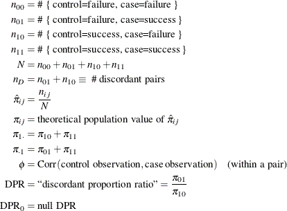
Power formulas are given here in terms of the discordant proportions ![]() and
and ![]() . If the input is specified in terms of
. If the input is specified in terms of ![]() , then it can be converted into values for
, then it can be converted into values for ![]() as follows:
as follows:
All McNemar tests covered in PROC POWER are conditional, meaning that ![]() is assumed fixed at its observed value.
is assumed fixed at its observed value.
For the usual ![]() , the hypotheses are
, the hypotheses are
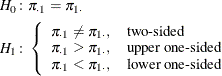
The test statistic for both tests covered in PROC POWER (DIST=EXACT_COND and DIST=NORMAL) is the McNemar statistic ![]() , which has the following form when
, which has the following form when ![]() :
:
For the conditional McNemar tests, this is equivalent to the square of the ![]() statistic for the test of a single proportion (normal approximation to binomial), where the proportion is
statistic for the test of a single proportion (normal approximation to binomial), where the proportion is ![]() , the null is 0.5, and “N” is
, the null is 0.5, and “N” is ![]() (see, for example, Schork and Williams 1980):
(see, for example, Schork and Williams 1980):
![\begin{align*} Z(X) & = \frac{n_{01} - n_ D (0.5)}{\left[ n_ D 0.5(1-0.5) \right]^\frac {1}{2}} \quad {\stackrel{\cdot }{\thicksim }} \; \mr {N}\left(\frac{n_ D^{\frac{1}{2}}(\frac{\pi _{01}}{\pi _{01}+\pi _{10}} - 0.5)}{\left[ 0.5(1-0.5) \right]^\frac {1}{2}}, \frac{\frac{\pi _{01}}{\pi _{01}+\pi _{10}} \left(1-\frac{\pi _{01}}{\pi _{01}+\pi _{10}}\right)}{0.5(1-0.5)}\right) \\ & = \frac{n_{01} - (n_{01} + n_{10}) (0.5)}{\left[ (n_{01} + n_{10}) 0.5(1-0.5) \right]^\frac {1}{2}} \\ & = \frac{n_{01} - n_{10}}{\left[ n_{01} + n_{10} \right]^\frac {1}{2}} \\ & = \sqrt {Q_{M_0}} \\ \end{align*}](images/statug_power0352.png)
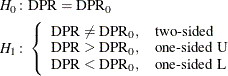
This can be generalized to a custom null for ![]() , which is equivalent to specifying a custom null DPR:
, which is equivalent to specifying a custom null DPR:
![\[ \left[\frac{\pi _{01}}{\pi _{01}+\pi _{10}} \right]_0 \equiv \left[ \frac{1}{1+\frac{1}{\frac{\pi _{01}}{\pi _{10}}}} \right]_0 \equiv \frac{1}{1+\frac{1}{\mr {DPR}_0}} \]](images/statug_power0353.png)
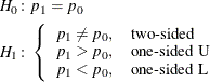
So, a conditional McNemar test (asymptotic or exact) with a custom null is equivalent to the test of a single proportion
![]() with a null value
with a null value ![]() , with a sample size of
, with a sample size of ![]() :
:
which is equivalent to
The general form of the test statistic is thus
The two most common conditional McNemar tests assume either the exact conditional distribution of ![]() (covered by the DIST=EXACT_COND analysis) or a standard normal distribution for
(covered by the DIST=EXACT_COND analysis) or a standard normal distribution for ![]() (covered by the DIST=NORMAL analysis).
(covered by the DIST=NORMAL analysis).
For DIST=EXACT_COND, the power is calculated assuming that the test is conducted by using the exact conditional distribution
of ![]() (conditional on
(conditional on ![]() ). The power is calculated by first computing the conditional power for each possible
). The power is calculated by first computing the conditional power for each possible ![]() . The unconditional power is computed as a weighted average over all possible outcomes of
. The unconditional power is computed as a weighted average over all possible outcomes of ![]() :
:
where ![]() , and
, and ![]() is calculated by using the exact method in the section Exact Test of a Binomial Proportion (TEST=EXACT).
is calculated by using the exact method in the section Exact Test of a Binomial Proportion (TEST=EXACT).
The achieved significance level, reported as “Actual Alpha” in the analysis, is computed in the same way except by using the actual alpha of the one-sample test in place of its power:
where ![]() is the actual alpha calculated by using the exact method in the section Exact Test of a Binomial Proportion (TEST=EXACT) with proportion
is the actual alpha calculated by using the exact method in the section Exact Test of a Binomial Proportion (TEST=EXACT) with proportion ![]() , null
, null ![]() , and sample size
, and sample size ![]() .
.
For DIST=NORMAL, power is calculated assuming the test is conducted by using the normal-approximate distribution of ![]() (conditional on
(conditional on ![]() ).
).
For the METHOD=EXACT option, the power is calculated in the same way as described in the section McNemar Exact Conditional Test (TEST=MCNEMAR DIST=EXACT_COND), except that ![]() is calculated by using the exact method in the section z Test for Binomial Proportion Using Null Variance (TEST=Z VAREST=NULL). The achieved significance level is calculated in the same way as described at the end of the section McNemar Exact Conditional Test (TEST=MCNEMAR DIST=EXACT_COND).
is calculated by using the exact method in the section z Test for Binomial Proportion Using Null Variance (TEST=Z VAREST=NULL). The achieved significance level is calculated in the same way as described at the end of the section McNemar Exact Conditional Test (TEST=MCNEMAR DIST=EXACT_COND).
For the METHOD=MIETTINEN option, approximate sample size for the one-sided cases is computed according to equation (5.6) in Miettinen (1968):
![\[ N = \frac{\left\{ z_{1-\alpha }(p_{10}+p_{01}) + z_{\mathit{power}} \left[(p_{10}+p_{01})^2 - \frac{1}{4}(p_{01}-p_{10})^2 (3+p_{10}+p_{01}) \right]^\frac {1}{2} \right\} ^2}{(p_{10}+p_{01}) (p_{01}-p_{10})^2} \]](images/statug_power0364.png)
Approximate power for the one-sided cases is computed by solving the sample size equation for power, and approximate power
for the two-sided case follows easily by summing the one-sided powers each at ![]() :
:
![\[ \mr {power} = \left\{ \begin{array}{ll} \Phi \left(\frac{(p_{01}-p_{10}) \left[N(p_{10}+p_{01})\right]^\frac {1}{2} - z_{1-\alpha }(p_{10}+p_{01})}{\left[ (p_{10}+p_{01})^2 - \frac{1}{4}(p_{01}-p_{10})^2 (3+p_{10}+p_{01}) \right]^\frac {1}{2}} \right), & \mbox{upper one-sided} \\ \Phi \left(\frac{-(p_{01}-p_{10}) \left[N(p_{10}+p_{01})\right]^\frac {1}{2} - z_{1-\alpha }(p_{10}+p_{01})}{\left[ (p_{10}+p_{01})^2 - \frac{1}{4}(p_{01}-p_{10})^2 (3+p_{10}+p_{01}) \right]^\frac {1}{2}} \right), & \mbox{lower one-sided} \\ \Phi \left(\frac{(p_{01}-p_{10}) \left[N(p_{10}+p_{01})\right]^\frac {1}{2} - z_{1-\frac{\alpha }{2}}(p_{10}+p_{01})}{\left[ (p_{10}+p_{01})^2 - \frac{1}{4}(p_{01}-p_{10})^2 (3+p_{10}+p_{01}) \right]^\frac {1}{2}} \right) + \\ \quad \Phi \left(\frac{-(p_{01}-p_{10}) \left[N(p_{10}+p_{01})\right]^\frac {1}{2} - z_{1-\frac{\alpha }{2}}(p_{10}+p_{01})}{\left[ (p_{10}+p_{01})^2 - \frac{1}{4}(p_{01}-p_{10})^2 (3+p_{10}+p_{01}) \right]^\frac {1}{2}} \right), & \mbox{two-sided} \\ \end{array} \right. \]](images/statug_power0366.png)
The two-sided solution for N is obtained by numerically inverting the power equation.
In general, compared to METHOD=CONNOR, the METHOD=MIETTINEN approximation tends to be slightly more accurate but can be slightly anticonservative in the sense of underestimating sample size and overestimating power (Lachin, 1992, p. 1250).
For the METHOD=CONNOR option, approximate sample size for the one-sided cases is computed according to equation (3) in Connor (1987):
![\[ N = \frac{\left\{ z_{1-\alpha }(p_{10}+p_{01})^\frac {1}{2} + z_{\mathit{power}} \left[p_{10}+p_{01} - (p_{01}-p_{10})^2 \right]^\frac {1}{2} \right\} ^2}{(p_{01}-p_{10})^2} \]](images/statug_power0367.png)
Approximate power for the one-sided cases is computed by solving the sample size equation for power, and approximate power
for the two-sided case follows easily by summing the one-sided powers each at ![]() :
:
![\[ \mr {power} = \left\{ \begin{array}{ll} \Phi \left( \frac{ (p_{01}-p_{10}) N^\frac {1}{2} - z_{1-\alpha }(p_{10}+p_{01})^\frac {1}{2}}{\left[ p_{10}+p_{01} - (p_{01}-p_{10})^2 \right]^\frac {1}{2}} \right), & \mbox{upper one-sided} \\ \Phi \left( \frac{ -(p_{01}-p_{10}) N^\frac {1}{2} - z_{1-\alpha }(p_{10}+p_{01})^\frac {1}{2}}{\left[ p_{10}+p_{01} - (p_{01}-p_{10})^2 \right]^\frac {1}{2}} \right), & \mbox{lower one-sided} \\ \Phi \left( \frac{ (p_{01}-p_{10}) N^\frac {1}{2} - z_{1-\frac{\alpha }{2}}(p_{10}+p_{01})^\frac {1}{2}}{\left[ p_{10}+p_{01} - (p_{01}-p_{10})^2 \right]^\frac {1}{2}} \right) + \\ \quad \Phi \left( \frac{ -(p_{01}-p_{10}) N^\frac {1}{2} - z_{1-\frac{\alpha }{2}}(p_{10}+p_{01})^\frac {1}{2}}{\left[ p_{10}+p_{01} - (p_{01}-p_{10})^2 \right]^\frac {1}{2}} \right), & \mbox{two-sided} \\ \end{array} \right. \]](images/statug_power0368.png)
The two-sided solution for N is obtained by numerically inverting the power equation.
In general, compared to METHOD=MIETTINEN, the METHOD=CONNOR approximation tends to be slightly less accurate but slightly conservative in the sense of overestimating sample size and underestimating power (Lachin, 1992, p. 1250).