The PLM Procedure

The following DATA step creates a data set from a randomized block experiment with a factorial treatment structure of factors
A and B:
data BlockDesign;
   input block a b y @@;
   datalines;
   1 1 1  56  1 1 2  41
   1 2 1  50  1 2 2  36
   1 3 1  39  1 3 2  35
   2 1 1  30  2 1 2  25
   2 2 1  36  2 2 2  28
   2 3 1  33  2 3 2  30
   3 1 1  32  3 1 2  24
   3 2 1  31  3 2 2  27
   3 3 1  15  3 3 2  19
   4 1 1  30  4 1 2  25
   4 2 1  35  4 2 2  30
   4 3 1  17  4 3 2  18
;
The GLM procedure is used in the following statements to fit the model and to create a source item store for the PLM procedure:
proc glm data=BlockDesign;
   class block a b;
   model y = block a b a*b / solution;
   store sasuser.BlockAnalysis / label='PLM: Getting Started';
run;
The CLASS statement identifies the variables Block, A, and B as classification variables. The MODEL statement specifies the response variable and the model effects. The block effect models the design effect, and the a, b, and a*b effects model the factorial treatment structure. The STORE statement requests that the context and results of this analysis
be saved to an item store named sasuser.BlockAnalysis. Because the SASUSER library is specified as the library name of the item store, the store will be available after the SAS session completes.
The optional label in the STORE statement identifies the store in subsequent analyses with the PLM procedure.
Note that having BlockDesign as the name of the output store would not create a conflict with the input data set name, because data sets and item stores
are saved as files of different types.
Figure 73.1 displays the results from the GLM procedure. The “Class Level Information” table shows the number of levels and their values for the three classification variables. The “Parameter Estimates” table shows the estimates and their standard errors along with t tests.
Figure 73.1: Class Variable Information, Fit Statistics, and Parameter Estimates
| Class Level Information | ||
|---|---|---|
| Class | Levels | Values |
| block | 4 | 1 2 3 4 |
| a | 3 | 1 2 3 |
| b | 2 | 1 2 |
| R-Square | Coeff Var | Root MSE | y Mean |
|---|---|---|---|
| 0.848966 | 15.05578 | 4.654747 | 30.91667 |
| Parameter | Estimate | Standard Error | t Value | Pr > |t| | |
|---|---|---|---|---|---|
| Intercept | 20.41666667 | B | 2.85043856 | 7.16 | <.0001 |
| block 1 | 17.00000000 | B | 2.68741925 | 6.33 | <.0001 |
| block 2 | 4.50000000 | B | 2.68741925 | 1.67 | 0.1148 |
| block 3 | -1.16666667 | B | 2.68741925 | -0.43 | 0.6704 |
| block 4 | 0.00000000 | B | . | . | . |
| a 1 | 3.25000000 | B | 3.29140294 | 0.99 | 0.3391 |
| a 2 | 4.75000000 | B | 3.29140294 | 1.44 | 0.1695 |
| a 3 | 0.00000000 | B | . | . | . |
| b 1 | 0.50000000 | B | 3.29140294 | 0.15 | 0.8813 |
| b 2 | 0.00000000 | B | . | . | . |
| a*b 1 1 | 7.75000000 | B | 4.65474668 | 1.66 | 0.1167 |
| a*b 1 2 | 0.00000000 | B | . | . | . |
| a*b 2 1 | 7.25000000 | B | 4.65474668 | 1.56 | 0.1402 |
| a*b 2 2 | 0.00000000 | B | . | . | . |
| a*b 3 1 | 0.00000000 | B | . | . | . |
| a*b 3 2 | 0.00000000 | B | . | . | . |
The following statements invoke the PLM procedure and use sasuser.BlockAnalysis as the source item store:
proc plm restore=sasuser.BlockAnalysis;
run;
These statements produce Figure 73.2. The “Store Information” table displays information that is gleaned from the source item store. For example, the store was created by the GLM procedure
at the indicated time and date, and the input data set for the analysis was WORK.BLOCKDESIGN. The label used earlier in the STORE statement of the GLM procedure also appears as a descriptor in Figure 73.2.
Figure 73.2: Default Information
| Store Information | |
|---|---|
| Item Store | SASUSER.BLOCKANALYSIS |
| Label | PLM: Getting Started |
| Data Set Created From | WORK.BLOCKDESIGN |
| Created By | PROC GLM |
| Date Created | 24OCT13:13:54:05 |
| Response Variable | y |
| Class Variables | block a b |
| Model Effects | Intercept block a b a*b |
| Class Level Information | ||
|---|---|---|
| Class | Levels | Values |
| block | 4 | 1 2 3 4 |
| a | 3 | 1 2 3 |
| b | 2 | 1 2 |
The “Store Information” table also echoes partial information about the variables and model effects that are used in the analysis. The “Class Level Information” table is produced by the PLM procedure by default whenever the model contains effects that depend on CLASS variables.
The following statements request a display of the fit statistics and the parameter estimates from the source item store and a test of the treatment main effects and their interactions:
proc plm restore=sasuser.BlockAnalysis;
   show fit parms;
   test a b a*b;
run;
The statements produce Figure 73.3. Notice that the estimates and standard errors in the “Parameter Estimates” table agree with the results displayed earlier by the GLM procedure, except for small differences in formatting.
Figure 73.3: Fit Statistics, Parameter Estimates, and Tests of Effects
| Fit Statistics | |
|---|---|
| MSE | 21.66667 |
| Error df | 15 |
| Parameter Estimates | |||||
|---|---|---|---|---|---|
| Effect | block | a | b | Estimate | Standard Error |
| Intercept | 20.4167 | 2.8504 | |||
| block | 1 | 17.0000 | 2.6874 | ||
| block | 2 | 4.5000 | 2.6874 | ||
| block | 3 | -1.1667 | 2.6874 | ||
| block | 4 | 0 | . | ||
| a | 1 | 3.2500 | 3.2914 | ||
| a | 2 | 4.7500 | 3.2914 | ||
| a | 3 | 0 | . | ||
| b | 1 | 0.5000 | 3.2914 | ||
| b | 2 | 0 | . | ||
| a*b | 1 | 1 | 7.7500 | 4.6547 | |
| a*b | 1 | 2 | 0 | . | |
| a*b | 2 | 1 | 7.2500 | 4.6547 | |
| a*b | 2 | 2 | 0 | . | |
| a*b | 3 | 1 | 0 | . | |
| a*b | 3 | 2 | 0 | . | |
| Type III Tests of Model Effects | ||||
|---|---|---|---|---|
| Effect | Num DF | Den DF | F Value | Pr > F |
| a | 2 | 15 | 7.54 | 0.0054 |
| b | 1 | 15 | 8.38 | 0.0111 |
| a*b | 2 | 15 | 1.74 | 0.2097 |
Since the main effects, but not the interaction are significant in this experiment, the subsequent analysis focuses on the
main effects, in particular on the effect of variable A.
The following statements request the least squares means of the A effect along with their pairwise differences:
proc plm restore=sasuser.BlockAnalysis seed=3;
   lsmeans     a         / diff;
   lsmestimate a -1 1,
                  1  1 -2 / uppertailed ftest;
run;
The LSMESTIMATE statement tests two linear combinations of the A least squares means: equality of the first two levels and whether the sum of the first two level effects equals twice the
effect of the third level. The FTEST option in the LSMESTIMATE statement requests a joint F test for this two-row contrast. The UPPERTAILED option requests that the F test also be carried out under one-sided order restrictions. Since F tests under order restrictions (chi-bar-square statistic) require a simulation-based approach for the calculation of p-values, the random number stream is initialized with a seed value through the SEED= option in the PROC PLM statement.
The results of the LSMEANS and the LSMESTIMATE statement are shown in Figure 73.4.
Figure 73.4: LS-Means Related Inference for A Effect
| a Least Squares Means | |||||
|---|---|---|---|---|---|
| a | Estimate | Standard Error | DF | t Value | Pr > |t| |
| 1 | 32.8750 | 1.6457 | 15 | 19.98 | <.0001 |
| 2 | 34.1250 | 1.6457 | 15 | 20.74 | <.0001 |
| 3 | 25.7500 | 1.6457 | 15 | 15.65 | <.0001 |
| Differences of a Least Squares Means | ||||||
|---|---|---|---|---|---|---|
| a | _a | Estimate | Standard Error | DF | t Value | Pr > |t| |
| 1 | 2 | -1.2500 | 2.3274 | 15 | -0.54 | 0.5991 |
| 1 | 3 | 7.1250 | 2.3274 | 15 | 3.06 | 0.0079 |
| 2 | 3 | 8.3750 | 2.3274 | 15 | 3.60 | 0.0026 |
| Least Squares Means Estimates | |||||||
|---|---|---|---|---|---|---|---|
| Effect | Label | Estimate | Standard Error | DF | t Value | Tails | Pr > t |
| a | Row 1 | 1.2500 | 2.3274 | 15 | 0.54 | Upper | 0.2995 |
| a | Row 2 | 15.5000 | 4.0311 | 15 | 3.85 | Upper | 0.0008 |
| F Test for Least Squares Means Estimates | ||||||
|---|---|---|---|---|---|---|
| Effect | Num DF | Den DF | F Value | Pr > F | ChiBarSq Value | Pr > ChiBarSq |
| a | 2 | 15 | 7.54 | 0.0054 | 15.07 | 0.0001 |
The least squares means for the three levels of variable A are 32.875, 34.125, and 25.75. The differences between the third level and the first and second levels are statistically
significant at the 5% level (p-values of 0.0079 and 0.0026, respectively). There is no significant difference between the first two levels. The first row
of the “Least Squares Means Estimates” table also displays the difference between the first two levels of factor A. Although the (absolute value of the) estimate and its standard error are identical to those in the “Differences of a Least Squares Means” table, the p-values do not agree because one-sided tests were requested in the LSMESTIMATE statement.
The “F Test” table in Figure 73.4 shows the two degree-of-freedom test for the linear combinations of the LS-means. The F value of 7.54 with p-value of 0.0054 represents the usual (two-sided) F test. Under the one-sided right-tailed order restriction imposed by the UPPERTAILED option, the ChiBarSq value of 15.07 represents the observed value of the chi-bar-square statistic of Silvapulle and Sen (2004). The associated p-value of 0.0001 was obtained by simulation.
Now suppose that you are interested in analyzing the relationship of the interaction cell means. (Typically this would not
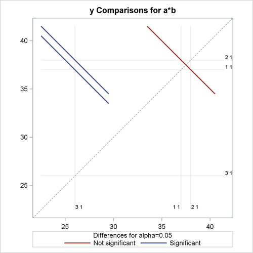
be the case in this example since the a*b interaction is not significant; see Figure 73.3.) The SLICE statement in the following PROC PLM run produces an F test of equality and all pair-wise differences of the interaction means for the subset (partition) where variable B is at level '1'. With ODS Graphics enabled, the pairwise differences are displayed in a diffogram.
ods graphics on;
proc plm restore=sasuser.BlockAnalysis;
   slice a*b / sliceby(b='1') diff;
run;
ods graphics off;
The results are shown in Figure 73.5. Since variable A has three levels, the test of equality of the A means at level '1' of B is a two-degree comparison. This comparison is statistically significant (p-value equals 0.0040). You can conclude that the three levels of A are not the same for the first level of B.
Figure 73.5: Results from Analyzing an Interaction Partition
| F Test for a*b Least Squares Means Slice |
||||
|---|---|---|---|---|
| Slice | Num DF | Den DF | F Value | Pr > F |
| b 1 | 2 | 15 | 8.18 | 0.0040 |
| Simple Differences of a*b Least Squares Means | |||||||
|---|---|---|---|---|---|---|---|
| Slice | a | _a | Estimate | Standard Error | DF | t Value | Pr > |t| |
| b 1 | 1 | 2 | -1.0000 | 3.2914 | 15 | -0.30 | 0.7654 |
| b 1 | 1 | 3 | 11.0000 | 3.2914 | 15 | 3.34 | 0.0045 |
| b 1 | 2 | 3 | 12.0000 | 3.2914 | 15 | 3.65 | 0.0024 |
The table of “Simple Differences” was produced by the DIFF option in the SLICE statement. As is the case with the marginal comparisons in Figure 73.4, there are significant differences against the third level of A if variable B is held fixed at '1'.
Figure 73.6 shows the diffogram that displays the three pairwise least squares mean differences and their significance. Each line segment corresponds to a comparison. It centers at the least squares means in the pair with its length corresponding to the projected width of a confidence interval for the difference. If the variable B is held fixed at '1', both the first two levels are significantly different from the third level, but the difference between the first and the second level is not significant.