The ROBUSTREG Procedure

M estimation in the context of regression was first introduced by Huber (1973) as a result of making the least squares approach robust. Although M estimators are not robust with respect to leverage points, they are popular in applications where leverage points are not an issue.
Instead of minimizing a sum of squares of the residuals, a Huber-type M estimator ![]() of
of ![]() minimizes a sum of less rapidly increasing functions of the residuals:
minimizes a sum of less rapidly increasing functions of the residuals:
where ![]() . For the ordinary least squares estimation,
. For the ordinary least squares estimation, ![]() is the square function,
is the square function, ![]() .
.
If ![]() is known, then by taking derivatives with respect to
is known, then by taking derivatives with respect to ![]() ,
, ![]() is also a solution of the system of p equations:
is also a solution of the system of p equations:
where ![]() . If
. If ![]() is convex,
is convex, ![]() is the unique solution.
is the unique solution.
The ROBUSTREG procedure solves this system by using iteratively reweighted least squares (IRLS). The weight function ![]() is defined as
is defined as
The ROBUSTREG procedure provides 10 kinds of weight functions through the WEIGHTFUNCTION= option in the MODEL statement. Each
weight function corresponds to a ![]() function. See the section Weight Functions for a complete discussion. You can specify the scale parameter
function. See the section Weight Functions for a complete discussion. You can specify the scale parameter ![]() with the SCALE= option in the PROC ROBUSTREG statement.
with the SCALE= option in the PROC ROBUSTREG statement.
If ![]() is unknown, both
is unknown, both ![]() and
and ![]() are estimated by minimizing the function
are estimated by minimizing the function
The algorithm proceeds by alternately improving ![]() in a location step and
in a location step and ![]() in a scale step.
in a scale step.
For the scale step, three methods are available to estimate ![]() , which you can select with the SCALE= option.
, which you can select with the SCALE= option.
-
(SCALE=HUBER <(D=d)>) Compute
 by the iteration
![\[ \left({\hat\sigma }^{(m+1)}\right)^2 = {1\over nh}\sum _{i=1}^ n \chi _ d \left( {r_ i\over {\hat\sigma }^{(m)}} \right) \left({\hat\sigma }^{(m)}\right)^2 \]](images/statug_rreg0053.png)
where
![\[ \chi _ d(x) = \left\{ \begin{array}{ll} x^2 / 2 & {\mbox{ if }} |x| < d \\ d^2 / 2 & {\mbox{ otherwise }} \end{array} \right. \]](images/statug_rreg0054.png)
is the Huber function and
 is the Huber constant (Huber, 1981, p. 179). You can specify d with the D=d option. By default, D=2.5.
-
(SCALE=TUKEY <(D=d)>) Compute
 by solving the supplementary equation
![\[ {1\over n-p}\sum _{i=1}^ n \chi _ d \left({r_ i \over \sigma }\right) = \beta \]](images/statug_rreg0057.png)
where
![\[ \chi _ d(x) = \left\{ \begin{array}{ll} {3x^2\over d^2} - {3x^4\over d^4} + {x^6\over d^6} & {\mbox{ if }} |x| < d \\ 1 & {\mbox{ otherwise }} \end{array} \right. \]](images/statug_rreg0058.png)
Here
 is Tukey’s bisquare function, and
  is the constant such that the solution is asymptotically consistent when
  (Hampel et al., 1986, p. 149). You can specify d with the D=d option. By default, D=2.5.
-
(SCALE=MED) Compute
by the iteration
![\[ {\hat\sigma }^{(m+1)} = {\mbox{median}} \left\{ |y_ i - \mb {x}_ i’ {\hat\btheta }^{(m)} |/ \beta _0, i=1,\ldots ,n \right\} \]](images/statug_rreg0062.png)
where
 is the constant such that the solution is asymptotically consistent when (Hampel et al., 1986, p. 312).
SCALE=MED is the default.
The basic algorithm for computing M estimates for regression is iteratively reweighted least squares (IRLS). As the name suggests, a weighted least squares fit is carried out inside an iteration loop. For each iteration, a set of weights for the observations is used in the least squares fit. The weights are constructed by applying a weight function to the current residuals. Initial weights are based on residuals from an initial fit. The ROBUSTREG procedure uses the unweighted least squares fit as a default initial fit. The iteration terminates when a convergence criterion is satisfied. The maximum number of iterations is set to 1,000. You can specify the weight function and the convergence criteria.
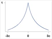
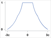
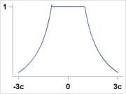
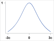
You can specify the weight function for M estimation with the WEIGHTFUNCTION= option. The ROBUSTREG procedure provides 10 weight functions. By default, the procedure uses the bisquare weight function. In most cases, M estimates are more sensitive to the parameters of these weight functions than to the type of the weight function. The median weight function is not stable and is seldom recommended in data analysis; it is included in the procedure for completeness. You can specify the parameters for these weight functions. Except for the Hampel and median weight functions, default values for these parameters are defined such that the corresponding M estimates have 95% asymptotic efficiency in the location model with the Gaussian distribution (Holland and Welsch, 1977).
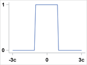
The following list shows the weight functions available. See Table 80.5 for the default values of the constants in these weight functions.
|
Andrews |
|
|
|
Bisquare |
|
|
|
Cauchy |
|
|
|
Fair |
|
|
|
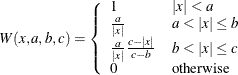
Hampel |
|
|
|
Huber |
|
|
|
Logistic |
|
|
|
Median |
|
|
|
Talworth |
|
|
|
Welsch |
|
|
The following convergence criteria are available in PROC ROBUSTREG:
-
relative change in the coefficients (CONVERGENCE= COEF)
-
relative change in the scaled residuals (CONVERGENCE= RESID)
-
relative change in weights (CONVERGENCE= WEIGHT)
You can specify the criteria with the CONVERGENCE= option in the PROC ROBUSTREG statement. The default is CONVERGENCE= COEF.
You can specify the precision of the convergence criterion with the EPS= suboption. The default is EPS=1E–8.
In addition to these convergence criteria, a convergence criterion based on scale-independent measure of the gradient is always checked. See Coleman et al. (1980) for more details. A warning is issued if this criterion is not satisfied.
The following three estimators of the asymptotic covariance of the robust estimator are available in PROC ROBUSTREG:
where ![]() is a correction factor and
is a correction factor and ![]() . See Huber (1981, p. 173) for more details.
. See Huber (1981, p. 173) for more details.
You can specify the asymptotic covariance estimate with the option ASYMPCOV= option. The ROBUSTREG procedure uses H1 as the default because of its simplicity and stability. Confidence intervals are computed from the diagonal elements of the estimated asymptotic covariance matrix.
The robust version of R-square is defined as
![\[ R^2 = {{\sum \rho \left({y_ i-{\hat\mu } \over {\hat s}}\right) - \sum \rho \left({y_ i-\mb {x}_ i’ {\hat\btheta } \over {\hat s}}\right) \over \sum \rho \left({y_ i-{\hat\mu } \over {\hat s}}\right)}} \]](images/statug_rreg0079.png)
and the robust deviance is defined as the optimal value of the objective function on the ![]() scale
scale
where ![]() ,
, ![]() is the M estimator of
is the M estimator of ![]() ,
, ![]() is the M estimator of location, and
is the M estimator of location, and ![]() is the M estimator of the scale parameter in the full model.
is the M estimator of the scale parameter in the full model.
Two tests are available in PROC ROBUSTREG for the canonical linear hypothesis
where q is the total number of parameters of the tested effects. The first test is a robust version of the F test, which is referred to as the ![]() test. Denote the M estimators in the full and reduced models as
test. Denote the M estimators in the full and reduced models as ![]() and
and ![]() , respectively. Let
, respectively. Let
|
|
|
|
|
|
|
|
with
The robust F test is based on the test statistic
Asymptotically ![]() under
under ![]() , where the standardization factor is
, where the standardization factor is ![]()
![]() and
and ![]() is the cumulative distribution function of the standard normal distribution. Large values of
is the cumulative distribution function of the standard normal distribution. Large values of ![]() are significant. This test is a special case of the general
are significant. This test is a special case of the general ![]() test of Hampel et al. (1986, Section 7.2).
test of Hampel et al. (1986, Section 7.2).
The second test is a robust version of the Wald test, which is referred to as ![]() test. The test uses a test statistic
test. The test uses a test statistic
where ![]() is the
is the ![]() block (corresponding to
block (corresponding to ![]() ) of the asymptotic covariance matrix of the M estimate
) of the asymptotic covariance matrix of the M estimate ![]() of
of ![]() in a p-parameter linear model.
in a p-parameter linear model.
Under ![]() , the statistic
, the statistic ![]() has an asymptotic
has an asymptotic ![]() distribution with q degrees of freedom. Large values of
distribution with q degrees of freedom. Large values of ![]() are significant. See Hampel et al. (1986, Chapter 7) for more details.
are significant. See Hampel et al. (1986, Chapter 7) for more details.
When M estimation is used, two criteria are available in PROC ROBUSTREG for model selection. The first criterion is a counterpart of the Akaike (1974) information criterion for robust regression (AICR); it is defined as
where ![]() ,
, ![]() is a robust estimate of
is a robust estimate of ![]() and
and ![]() is the M estimator with p-dimensional design matrix.
is the M estimator with p-dimensional design matrix.
As with AIC, ![]() is the weight of the penalty for dimensions. The ROBUSTREG procedure uses
is the weight of the penalty for dimensions. The ROBUSTREG procedure uses ![]() (Ronchetti, 1985) and estimates it by using the final robust residuals.
(Ronchetti, 1985) and estimates it by using the final robust residuals.
The second criterion is a robust version of the Schwarz information criteria (BICR); it is defined as