The QUANTREG Procedure

This example is patterned after a quantile regression analysis of covariates associated with birth weight that was carried out by Koenker and Hallock (2001). Their study used a subset of the June 1997 Detailed Natality Data published by the National Center for Health Statistics and demonstrated that conditional quantile functions provide more complete information about the covariate effects than ordinary least squares regression.
This example is based on Koenker and Hallock (2001); Abreveya (2001); it uses data for live, singleton births to mothers in the United States who were recorded as black or white, and who were between the ages of 18 and 45. For convenience, this example uses 50,000 observations, which were randomly selected from the qualified observations. Observations with missing data for any of the variables were deleted.
The following table describes the variables in the data.
|
Variable |
Description |
|
|---|---|---|
|
|
Infant’s birth weight |
|
|
|
Indicator of black mother |
|
|
|
Indicator of married mother |
|
|
|
Indicator of boy |
|
|
|
Prenatal visit: 0 = no visit, 1 = visit in second trimester, |
|
|
2 = visit in last trimester, 3 = visit in first trimester |
||
|
|
Mother’s education level: 0 = high school, 1 = some college, |
|
|
2 = college, 3 = less than high school |
||
|
|
Indicator of smoking mother |
|
|
|
Number of cigarettes smoked per day |
|
|
|
Mother’s age |
|
|
|
Mother’s weight gain during pregnancy |
There are four levels of education of the mother. By default, the QUANTREG procedure treats the highest level (3 - less than high school) as a reference level. The regression coefficients of other levels measure the effect relative to this level. Likewise, there are four levels of prenatal medical care of the mother, and a first visit in the first trimester serves as the reference level. These two variables are treated as classification variables in the model.
The following statements fit a regression model for 19 quantiles of birth weight, which are evenly spaced in the interval
![]() . The model includes linear and quadratic effects for the age of the mother and for weight gain during pregnancy.
. The model includes linear and quadratic effects for the age of the mother and for weight gain during pregnancy.
ods graphics on;

proc quantreg ci=sparsity/iid algorithm=interior(tolerance=5.e-4)
              data=sashelp.bweight;
   class visit ed;
   model weight = black married boy visit ed smoke
                  cigsper mom_age mom_age*mom_age
                  m_wtgain m_wtgain*m_wtgain /
                  quantile= 0.05 to 0.95 by 0.05
                  plot=quantplot;
run;
Output 77.3.1: Model Information and Summary Statistics
| BMI Percentiles for Men: 2-80 Years Old |
| Model Information | |
|---|---|
| Data Set | SASHELP.BWEIGHT |
| Dependent Variable | weight |
| Number of Independent Variables | 9 |
| Number of Continuous Independent Variables | 7 |
| Number of Class Independent Variables | 2 |
| Number of Observations | 50000 |
| Optimization Algorithm | Interior |
| Method for Confidence Limits | Sparsity |
| Summary Statistics | ||||||
|---|---|---|---|---|---|---|
| Variable | Q1 | Median | Q3 | Mean | Standard Deviation |
MAD |
| black | 0 | 0 | 0 | 0.1628 | 0.3692 | 0 |
| married | 0 | 1.0000 | 1.0000 | 0.7126 | 0.4525 | 0 |
| boy | 0 | 1.0000 | 1.0000 | 0.5158 | 0.4998 | 0 |
| smoke | 0 | 0 | 0 | 0.1307 | 0.3370 | 0 |
| cigsper | 0 | 0 | 0 | 1.4766 | 4.6541 | 0 |
| mom_age | -4.0000 | 0 | 5.0000 | 0.4161 | 5.7285 | 5.9304 |
| mom_age*mom_age | 4.0000 | 16.0000 | 49.0000 | 32.9877 | 39.2861 | 22.2390 |
| m_wtgain | -8.0000 | 0 | 9.0000 | 0.7092 | 12.8761 | 11.8608 |
| m_wtgain*m_wtgain | 16.0000 | 64.0000 | 196.0 | 166.3 | 298.8 | 88.9561 |
| weight | 3062.0 | 3402.0 | 3720.0 | 3370.8 | 566.4 | 504.1 |
Output 77.3.1 displays the model information and summary statistics for the variables in the model.
Among the 11 independent variables, Black, Married, Boy, and Smoke are binary variables. For these variables, the mean represents the proportion in the category. The two continuous variables,
Mom_Age and M_WtGain, are centered at their medians, which are 27 and 30, respectively.
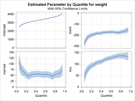
The quantile plots for the intercept and the other 15 factors with nonzero degree of freedom are shown in the following four panels. In each plot, the regression coefficient at a given quantile indicates the effect on birth weight of a unit change in that factor, assuming that the other factors are fixed. The bands represent 95% confidence intervals.
Although the data set used here is a subset of the Natality data set, the results are quite similar to those of Koenker and Hallock (2001) for the full data set.
In Output 77.3.2, the first plot is for the intercept. As explained by Koenker and Hallock (2001), the intercept “may be interpreted as the estimated conditional quantile function of the birth-weight distribution of a girl born to an unmarried, white mother with less than a high school education, who is 27 years old and had a weight gain of 30 pounds, didn’t smoke, and had her first prenatal visit in the first trimester of the pregnancy.”
The second plot shows that infants born to black mothers weigh less than infants born to white mothers, especially in the lower tail of the birth-weight distribution. The third plot shows that marital status has a large positive effect on birth weight, especially in the lower tail. The fourth plot shows that boys weigh more than girls for any chosen quantile; this difference is smaller in the lower quantiles of the distribution.
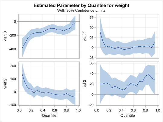
In Output 77.3.3, the first three plots deal with prenatal care. Compared with babies born to mothers who had a prenatal visit in the first trimester, babies born to mothers who received no prenatal care weigh less, especially in the lower quantiles of the birth-weight distributions. As noted by Koenker and Hallock (2001), “babies born to mothers who delayed prenatal visits until the second or third trimester have substantially higher birthweights in the lower tail than mothers who had a prenatal visit in the first trimester. This might be interpreted as the self-selection effect of mothers confident about favorable outcomes.”
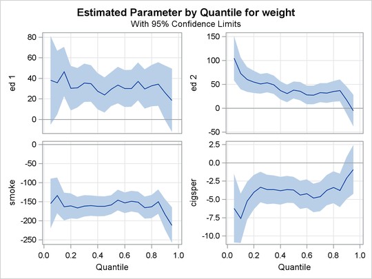
The fourth plot in Output 77.3.3 and the first two plots in Output 77.3.4 are for variables related to education. Education beyond high school is associated with a positive effect on birth weight. The effect of high school education is uniformly around 15 grams across the entire birth-weight distribution (this is a pure location shift effect), while the effect of some college and college education is more positive in the lower quantiles than the upper quantiles.
The remaining two plots in Output 77.3.4 show that smoking is associated with a large negative effect on birth weight.
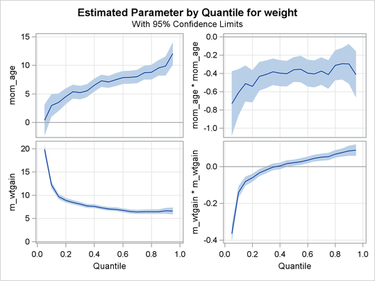
The linear and quadratic effects for the two continuous variables are shown in Output 77.3.5. Both of these variables are centered at their median. At the lower quantiles, the quadratic effect of the mother’s age is more concave. The optimal age at the first quantile is about 33, and the optimal age at the third quantile is about 38. The effect of the mother’s weight gain is clearly positive, as indicated by the narrow confidence bands for both linear and quadratic coefficients.
See Koenker and Hallock (2001) for more details about the covariate effects discovered with quantile regression.