The PLM Procedure

This example demonstrates how you can use PROC PLM to perform posterior inference from a Bayesian analysis. The data for this
example are taken from Weisberg (1985) and concern the effect of small electrical currents on farm animals. The ultimate goal of the experiment was to understand
the effects of high-voltage power lines on livestock and to better protect farm animals. Seven cows and six shock intensities
were used in two experiments. In one experiment, each cow was given 30 electrical shocks with five at each shock intensity
in random order. The number of shock responses was recorded for each cow at each shock level. The experiment was then repeated
to investigate whether the response diminished due to fatigue of cows, or due to learning. So each cow received a total of
60 shocks. For the following analysis, the cow difference is ignored. The following DATA step lists the data where the variable
current represents the shock level, the variable response represents the number of shock responses, the variable trial represents the total number of trials at each shock level, and the variable experiment represents the experiment number (1 for the initial experiment and 2 for the repeated one):
data cow;
   input current response trial experiment;
   datalines;
0  0 35 1
0  0 35 2
1  6 35 1
1  3 35 2
2 13 35 1
2  8 35 2
3 26 35 1
3 21 35 2
4 33 35 1
4 27 35 2
5 34 35 1
5 29 35 2
;
Suppose you are interested in modeling the distribution of the shock response based on the level of the current and the experiment
number. You can use the GENMOD procedure to fit a frequentist logistic model for the data. However, if you have some prior
information about parameter estimates, you can fit a Bayesian logistic regression model to take this prior information into
account. In this case, suppose you believe the logit of response has a positive association with the shock level but you are uncertain about the ranges of other regression coefficients.
To incorporate this prior information in the regression model, you can use the following statements:
data prior;
   input _type_$ current;
   datalines;
mean 100
var   50
;
proc genmod data=cow;
   class experiment;
   bayes coeffprior=normal(input=prior) seed=1;
   model response/trial = current|experiment / dist=binomial;
   store cowgmd;
   title 'Bayesian Logistic Model on Cow';
run;
The DATA step creates a data set prior that specifies the prior distribution for the variable current, which in this case is a normal distribution with mean 100 and variance 50. This reflects a rough belief in a positive coefficient
in a moderate range for current. The prior distribution parameters are not specified for experiment and the interaction between experiment and current, and so PROC GENMOD assigns a default prior for them, which is a normal distribution with mean 0 and variance 1E6.
The BAYES statement in PROC GENMOD specifies that the regression coefficients follow a normal distribution with mean and variance
specified in the input data set named prior. It also specifies 1 as the seed for the random number generator in the simulation of the posterior sample. The MODEL statement
requests a logistic regression model with a logit link. The STORE statement requests that the fitted results be saved into
an item store named cowgmd.
The convergence diagnostics in the output of PROC GENMOD indicate that the Markov chain has converged. Output 69.4.1 displays summaries on the posterior sample of the regression coefficients. The posterior mean for the intercept is –3.5857
with a 95% HPD interval ![]() . The posterior mean of the coefficient for
. The posterior mean of the coefficient for current is 1.1893 with a 95% HPD interval ![]() , which indicates a positive association between the logit of
, which indicates a positive association between the logit of response and the shock level. Further investigation about whether shock reaction was different between two experiment is warranted.
Output 69.4.1: Posterior Summaries on the Bayesian Logistic Model
| Bayesian Logistic Model on Cow |
| Posterior Summaries | ||||||
|---|---|---|---|---|---|---|
| Parameter | N | Mean | Standard Deviation |
Percentiles | ||
| 25% | 50% | 75% | ||||
| Intercept | 10000 | -3.6047 | 0.4906 | -3.9281 | -3.5842 | -3.2679 |
| current | 10000 | 1.1966 | 0.1561 | 1.0873 | 1.1927 | 1.2996 |
| experiment1 | 10000 | 0.0350 | 0.7014 | -0.4206 | 0.0347 | 0.4987 |
| experiment1current | 10000 | 0.3574 | 0.2503 | 0.1906 | 0.3520 | 0.5235 |
| Posterior Intervals | |||||
|---|---|---|---|---|---|
| Parameter | Alpha | Equal-Tail Interval | HPD Interval | ||
| Intercept | 0.050 | -4.6233 | -2.7074 | -4.5611 | -2.6581 |
| current | 0.050 | 0.9073 | 1.5152 | 0.9028 | 1.5064 |
| experiment1 | 0.050 | -1.3651 | 1.4004 | -1.2995 | 1.4370 |
| experiment1current | 0.050 | -0.1293 | 0.8580 | -0.1287 | 0.8580 |
Bayesian model fitting typically involves a large amount of simulation. Using the item store and PROC PLM, you do not need to refit the model to perform further posterior inference. Suppose you want to determine whether the shock reaction for the current level is different between the two experiments. You can use PROC PLM with the ESTIMATE statement in the following statements:
proc plm restore=cowgmd;
   estimate
   'Diff at current 0' experiment 1 -1 current*experiment [1, 0 1] [-1, 0 2],
   'Diff at current 1' experiment 1 -1 current*experiment [1, 1 1] [-1, 1 2],
   'Diff at current 2' experiment 1 -1 current*experiment [1, 2 1] [-1, 2 2],
   'Diff at current 3' experiment 1 -1 current*experiment [1, 3 1] [-1, 3 2],
   'Diff at current 4' experiment 1 -1 current*experiment [1, 4 1] [-1, 4 2],
   'Diff at current 5' experiment 1 -1 current*experiment [1, 5 1] [-1, 5 2]
    / exp cl;
run;
Each line in the ESTIMATE statement compares the fits between the two groups at each current level. The nonpositional syntax
is used for the interaction effect current*experiment. For example, the first line requests coefficient 1 for the interaction effect at current level 0 for the initial experiment,
and coefficient –1 for the effect at current level 0 for the repeated experiment. The two terms are then added to derive the
difference. For more details about the nonpositional syntax, see Positional and Nonpositional Syntax for Coefficients in Linear Functions of Chapter 19: Shared Concepts and Topics.
The EXP option exponentiates log odds ratios to produce odds ratios. The CL option requests that confidence limits be constructed for both log odds ratios and odds ratios. Output 69.4.2 lists the posterior sample estimates for differences between experiments at different current levels.
Output 69.4.2: Comparisons between Experiments at Different Current Levels
| Bayesian Logistic Model on Cow |
| Sample Estimates | ||||||||||||||||
|---|---|---|---|---|---|---|---|---|---|---|---|---|---|---|---|---|
| Label | N | Estimate | Standard Deviation | Percentiles | Alpha | Lower HPD | Upper HPD | Exponentiated | Standard Deviation of Exponentiated |
Percentiles for Exponentiated |
Lower HPD of Exponentiated |
Upper HPD of Exponentiated |
||||
| 25th | 50th | 75th | 25th | 50th | 75th | |||||||||||
| Diff at current 0 | 10000 | 0.03500 | 0.7014 | -0.4206 | 0.0347 | 0.4987 | 0.05 | -1.2995 | 1.4370 | 1.3258 | 1.080632 | 0.6566 | 1.0353 | 1.6466 | 0.1263 | 3.3077 |
| Diff at current 1 | 10000 | 0.3924 | 0.4865 | 0.0700 | 0.3884 | 0.7096 | 0.05 | -0.5287 | 1.3599 | 1.6672 | 0.873185 | 1.0725 | 1.4746 | 2.0331 | 0.3809 | 3.3011 |
| Diff at current 2 | 10000 | 0.7498 | 0.3266 | 0.5283 | 0.7468 | 0.9719 | 0.05 | 0.1300 | 1.3827 | 2.2328 | 0.753450 | 1.6961 | 2.1101 | 2.6429 | 1.0081 | 3.7135 |
| Diff at current 3 | 10000 | 1.1072 | 0.3194 | 0.8901 | 1.1001 | 1.3220 | 0.05 | 0.4772 | 1.7182 | 3.1863 | 1.068673 | 2.4353 | 3.0045 | 3.7509 | 1.3990 | 5.1655 |
| Diff at current 4 | 10000 | 1.4646 | 0.4718 | 1.1387 | 1.4559 | 1.7756 | 0.05 | 0.5369 | 2.3694 | 4.8511 | 2.562732 | 3.1227 | 4.2885 | 5.9040 | 1.3083 | 9.6902 |
| Diff at current 5 | 10000 | 1.8219 | 0.6844 | 1.3508 | 1.8079 | 2.2601 | 0.05 | 0.4881 | 3.1505 | 7.8941 | 6.668085 | 3.8606 | 6.0976 | 9.5838 | 0.9081 | 19.4638 |
The sample statistics are constructed from the posterior sample saved in the item store cowgmd. From the output, the odds of a cow showing shock reaction at level 0 in the initial experiment is 1.2811 (with a 95% HPD
interval (0.07387, 3.1001)) times the odds in the repeated experiment. The HPD interval for the odds ratio is constructed
based on the mean and variance of the sample of the exponentiated log odds ratios, instead of based on the exponentiated mean
and variance of the posterior sample of log odds ratios. The HPD interval suggests that there is not much evidence that the
cows responded differently at current level 0 between the two experiments. Similar conclusions can be drawn for current level
1, 2, and 5. However, there is strong evidence that cows responded differently at current level 3 and 4 between the two experiments.
The possible explanation is that, if the current level is so small that cows could hardly feel it or the current level is
so strong that cows could hardly bear it, cows would respond consistently in the two experiment. If the current level is moderate,
cows might get used to it and their response diminished in the repeated experiment.
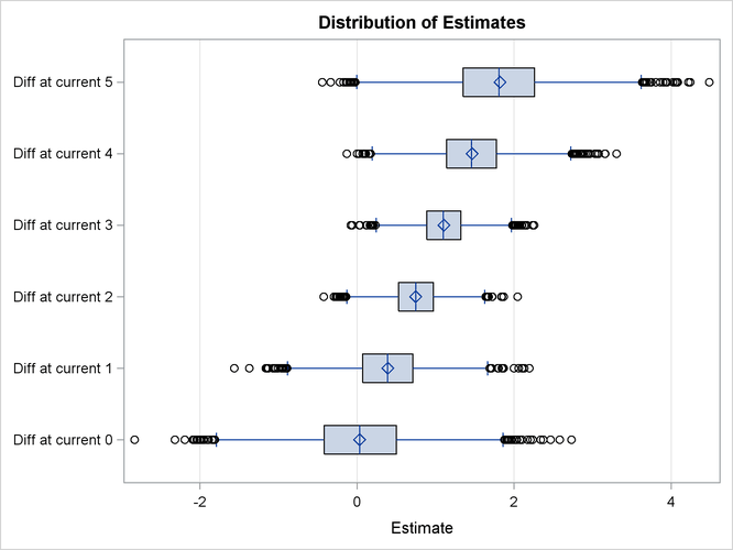
You can visualize the distribution of the posterior sample of log odds ratios by specifying the PLOTS= option in the ESTIMATE statement. In the following statements, ODS Graphics is enabled by the ODS GRAPHICS ON statement, the PLOTS=BOXPLOT option requests a box plot of posterior distribution of log odds ratios. The suboption ORIENT=HORIZONTAL specifies a horizontal orientation of the boxes.
ods graphics on;
proc plm restore=cowgmd;
   estimate
   'Diff at current 0' experiment 1 -1 current*experiment [1, 0 1] [-1, 0 2],
   'Diff at current 1' experiment 1 -1 current*experiment [1, 1 1] [-1, 1 2],
   'Diff at current 2' experiment 1 -1 current*experiment [1, 2 1] [-1, 2 2],
   'Diff at current 3' experiment 1 -1 current*experiment [1, 3 1] [-1, 3 2],
   'Diff at current 4' experiment 1 -1 current*experiment [1, 4 1] [-1, 4 2],
   'Diff at current 5' experiment 1 -1 current*experiment [1, 5 1] [-1, 5 2]
    / plots=boxplot(orient=horizontal);
run;
ods graphics off;
Output 69.4.3 displays the box plot of the posterior sample of log odds ratios. The two boxes for differences at current level 3 and 4 show that the corresponding log odds ratios are significantly larger than the reference value x = 0. This indicate that there is obvious evidence that the probability of cow response is larger in the initial experiment than in the repeated one at the two current levels. The other four boxes show that the corresponding log odds ratios are not significantly different from 0, which suggests that there is no obvious reaction difference at current level 0, 1, 2, and 5 between the two experiments.