The HPMIXED Procedure

RANDOM Statement

RANDOM random-effects </ options> ;

The RANDOM statement defines the random effects in the mixed model. It can be used to specify traditional variance component models (as in the VARCOMP procedure) and to specify random coefficients. The random effects can be classification or continuous. Multiple RANDOM statements are possible. Random effects specified in a RANDOM statement could be correlated with each other for certain types of covariance structures (see the TYPE= option). It is, however, assumed that random effects specified using different RANDOM statements are not correlated.

Using notation from the section Model Assumptions, the purpose of the RANDOM statement is to define the $\bZ$ matrix of the mixed model, the random effects in the $\bgamma$ vector, and the structure of $\bG$ . The $\bZ$ matrix is constructed exactly like the $\bX$ matrix for the fixed effects, and the $\bG$ matrix is constructed to correspond to the effects constituting $\bZ$ . The structure of $\bG$ is defined by using the TYPE= option.

You can specify INTERCEPT (or INT) as a random effect. PROC HPMIXED does not include the intercept in the RANDOM statement by default, as it does in the MODEL statement.

You can specify the following options in the RANDOM statement after a slash (/).

ALPHA=number

requests that a t-type confidence interval with confidence level $1-\mr {\Argument{number}}$ be constructed for the predictors of random effects in this statement. The value of number must be between 0 and 1 exclusively; the default is 0.05. Specifying the ALPHA= option implies the CL option.

CL

requests that t-type confidence limits be constructed for each of the predictors of random effects in this statement. The confidence level is 0.95 by default; this can be changed with the ALPHA= option. The CL option implies the SOLUTION option.

GROUP=effect

defines an effect specifying heterogeneity in the covariance structure of $\bG$ . All observations having the same level of the group effect have the same covariance parameters. Each new level of the group effect produces a new set of covariance parameters with the same structure as the original group. You should exercise caution in defining the group effect, because strange covariance patterns can result from its misuse. Also, the group effect can greatly increase the number of estimated covariance parameters, which can adversely affect the optimization process.

Continuous variables are permitted as arguments to the GROUP= option. PROC HPMIXED does not sort by the values of the continuous variable; rather, it considers the data to be from a new group whenever the value of the continuous variable changes from the previous observation. Using a continuous variable decreases execution time for models with a large number of groups and also prevents the production of a large “Class Levels Information” table.

NOFULLZ

eliminates the columns in $\bZ$ corresponding to missing levels of random effects involving CLASS variables. By default, these columns are included in $\bZ$ . It is sufficient to specify the NOFULLZ option in any RANDOM statement.

SOLUTION

requests that the solution for the random-effects parameters be produced. Using notation from the section Model Assumptions, these estimates are the empirical best linear unbiased predictors (BLUPs) 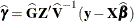$\widehat{\bgamma } = \widehat{\bG }\bZ ’\widehat{\bV }^{-1}(\mb {y} - \bX \widehat{\bbeta })$ . They can be useful for comparing the random effects from different experimental units and can also be treated as residuals in performing diagnostics for your mixed model.

The numbers displayed in the SE Pred column of the “Solution for Random Effects” table are not the standard errors of the $\widehat{\bgamma }$ displayed in the Estimate column; rather, they are the standard errors of predictions $\widehat{\bgamma }_ i - \bgamma _ i$ , where $\widehat{\bgamma }_ i$ is the ith BLUP and $\bgamma _ i$ is the ith random-effect parameter.

SUBJECT=effect

identifies the subjects in your mixed model. Complete independence is assumed across subjects; thus, for the RANDOM statement, the SUBJECT= option produces a block-diagonal structure in $\bG$ with identical blocks. The $\bZ$ matrix is modified to accommodate this block-diagonality. In fact, specifying a subject effect is equivalent to nesting all other effects in the RANDOM statement within the subject effect.

Continuous variables are permitted as arguments to the SUBJECT= option. PROC HPMIXED does not sort by the values of the continuous variable; rather, it considers the data to be from a new subject whenever the value of the continuous variable changes from the previous observation. Using a continuous variable decreases execution time for models with a large number of subjects and also prevents the production of a large “Class Levels Information” table.

TYPE=covariance-structure

specifies the structure of the covariance matrix $\bG$ for random effects. The default structure is VC.

If you want different covariance structures in different parts of $\bG$ , you must use multiple RANDOM statements with different TYPE= options.

Valid values for covariance-structure are listed in Table 46.8. Examples are shown in Table 46.9.

Table 46.8: Covariance Structures

Structure	Description	Parameters	element
AR(1)	Autoregressive(1)	2	$\sigma ^2\rho ^{\|i-j\|}$
CHOL	Cholesky root		$l_{ij}$
CS	Compound symmetry (CS)	2	$\sigma _1 + \sigma ^2 1(i = j)$
CSH	Heterogeneous CS		$\sigma _ i\sigma _ j[\rho 1(i \neq j)+ 1(i=j)]$
UC	Uniform correlation (UC)	2	$\sigma ^2[\rho 1(i \neq j) + 1(i=j)]$
UCH	Heterogeneous UC		$\sigma _ i\sigma _ j[\rho 1(i \neq j) + 1(i=j)]$
UN	Unstructured		$\sigma _{ij}$
VC	Variance components	q	$\sigma ^2_ k 1(i=j)$
			and i,j correspond to kth effect

In Table 46.8, t is the overall dimension of the covariance matrix, and equals 1 when A is true and 0 otherwise. For example, 1(i = j) equals 1 when i = j and equals 0 otherwise. TYPE=UCH is the same as TYPE=CSH.

Table 46.9 lists some examples of the structures in Table 46.8.

Table 46.9: Covariance Structure Examples

Description	Structure	Example
First-order autoregressive	AR(1)	$\sigma ^2\begin{bmatrix} 1 & \rho & \rho ^2 & \rho ^3 \\ \rho & 1 & \rho & \rho ^2 \\ \rho ^2 & \rho & 1 & \rho \\ \rho ^3 & \rho ^2 & \rho & 1 \end{bmatrix}$
Cholesky root	CHOL	$\left[\begin{array}{llll} l_{11} & 0 & 0 & 0 \\ l_{21} & l_{22} & 0 & 0 \\ l_{31} & l_{32} & l_{33} & 0 \\ l_{41} & l_{42} & l_{43} & l_{44} \end{array}\right] \left[\begin{array}{llll} l_{11} & l_{21} & l_{31} & l_{41} \\ 0 & l_{22} & l_{32} & l_{42} \\ 0 & 0 & l_{33} & l_{43} \\ 0 & 0 & 0 & l_{44} \end{array} \right]$
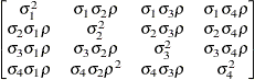
Compound symmetry	CS	$\begin{bmatrix} \sigma ^2 + \sigma _1 & \sigma _1 & \sigma _1 & \sigma _1 \\ \sigma _1 & \sigma ^2 + \sigma _1 & \sigma _1 & \sigma _1 \\ \sigma _1 & \sigma _1 & \sigma ^2 + \sigma _1 & \sigma _1 \\ \sigma _1 & \sigma _1 & \sigma _1 & \sigma ^2 + \sigma _1 \end{bmatrix}$
Uniform correlation	UC	$\sigma ^2\begin{bmatrix} 1 & \rho & \rho & \rho \\ \rho & 1 & \rho & \rho \\ \rho & \rho & 1 & \rho \\ \rho & \rho & \rho & 1 \end{bmatrix}$
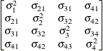
Heterogeneous UC	UCH	$\begin{bmatrix} \sigma _1^2 & \sigma _1\sigma _2\rho & \sigma _1\sigma _3\rho & \sigma _1\sigma _4\rho \\ \sigma _2\sigma _1\rho & \sigma _2^2 & \sigma _2\sigma _3\rho & \sigma _2\sigma _4\rho \\ \sigma _3\sigma _1\rho & \sigma _3\sigma _2\rho & \sigma _3^2 & \sigma _3\sigma _4\rho \\ \sigma _4\sigma _1\rho & \sigma _4\sigma _2\rho ^2 & \sigma _4\sigma _3\rho & \sigma _4^2 \end{bmatrix}$
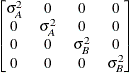
Unstructured	UN	$\begin{bmatrix} \sigma _1^2 & \sigma _{21} & \sigma _{31} & \sigma _{41} \\ \sigma _{21} & \sigma _2^2 & \sigma _{32} & \sigma _{42} \\ \sigma _{31} & \sigma _{32} & \sigma _3^2 & \sigma _{34} \\ \sigma _{41} & \sigma _{42} & \sigma _{43} & \sigma _4^2 \end{bmatrix}$
Variance components	VC (default)	$\begin{bmatrix} \sigma _{A}^{2} & 0 & 0 & 0 \\ 0 & \sigma _{A}^{2} & 0 & 0 \\ 0 & 0 & \sigma _{B}^{2} & 0 \\ 0 & 0 & 0 & \sigma _{B}^{2} \end{bmatrix}$

The variances and covariances in the formulas that follow in the TYPE= descriptions are expressed in terms of generic random variables $\xi _ i$ and $\xi _ j$ . They represent random effects for which the $\bG$ matrices are constructed.

The following list provides some further information about these covariance structures:

TYPE=AR(1)

specifies a first-order autoregressive structure,

$\mr {Cov}\left[\xi _ i,\xi _ j\right] = \sigma ^2 \rho ^{|i - j|}$

The values i and j are derived for the ith and jth observations, respectively. For example, in the following statements the values correspond to the class levels for the time effect of the ith and jth observation within a particular subject:

proc hpmixed;
   class time patient;
   model y = x x*x;
   random time / sub=patient type=ar(1);
run;

PROC HPMIXED imposes the constraint $|\rho | < 1$ for stationarity.

TYPE=CHOL

specifies an unstructured variance-covariance matrix parameterized through its Cholesky root. All diagonal values are constrained to be positive. This parameterization guarantees a positive definite covariance matrix. For example, a $2 \times 2$ unstructured covariance matrix can be written as

$\mr {Var}[\bxi ] = \left[ \begin{array}{cc} \sigma ^2_1 & \sigma _{21} \\ \sigma _{21} & \sigma ^2_2 \end{array} \right]$

Without imposing constraints on the three parameters, there is no guarantee that the estimated variance matrix is positive definite. Even if $\sigma ^2_1$ and $\sigma ^2_2$ are nonzero, a large value for $\sigma _{21}$ can lead to a negative eigenvalue of $\mr {Var}[\bxi ]$ . The Cholesky root of a positive definite matrix $\bA$ is a lower triangular matrix $\bL$ such that $\bL \bL ’ = \bA$ . The Cholesky root of the above $2 \times 2$ matrix can be written as

$\mb {L} = \left[ \begin{array}{cc} l_{11} & 0 \\ l_{21} & l_{22} \end{array} \right]$

The elements of the unstructured variance matrix are then simply $\sigma ^2_1 = l_{11}^2$ , $\sigma _{21} = l_{21} l_{11}$ , and $\sigma ^2_2 = l_{21}^2 + l_{22}^2$ . Similar operations yield the generalization to covariance matrices of higher orders.

For example, the following statements model the covariance matrix of each subject as an unstructured matrix:

proc hpmixed;
   class sub;
   model y = x;
   random  time / sub=patient type=chol;
run;

The HPMIXED procedure constrains the diagonal elements of the Cholesky root to be positive. This guarantees that the structure is positive definite.

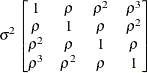
TYPE=CS

specifies the compound-symmetry structure, which has constant variance and constant covariance

$\mr {Cov}\left[\xi _ i,\xi _ j\right] = \left\{ \begin{array}{lc} \sigma ^2 + \sigma _1 & i=j \\ \sigma _1 & i \not= j \end{array} \right.$

Under compound-symmetry, the $\bG$ matrix is of form $\sigma ^2\bI + \sigma _1\bJ$ . The variance parameter $\sigma ^2$ is constrained to be positive, and the covariance parameter $\sigma _1$ is constrained to be greater than $-\sigma ^2/t$ where t is the dimension of the structure. This guarantees the structure is positive definite. The compound-symmetry structure arises naturally with nested random effects, such as when a subsampling error is nested within an experimental error.

TYPE=CSH

specifies the heterogeneous compound-symmetry structure. This structure has a different variance parameter for each diagonal element, and it uses the square roots of these parameters in the off-diagonal entries. In Table 46.8, $\sigma ^2_ i$ is the ith variance parameter that satisfies $\sigma ^2_ i > 0$ , and $\rho$ is the correlation parameter that satisfies $\rho >-1/(t-1)$ , where t is the dimension of the structure. This guarantees that the structure is positive definite.

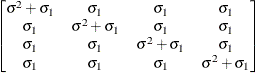
TYPE=UC

specifies the uniform correlation structure, which has constant variance and constant correlation

$\mr {Cov}\left[\xi _ i,\xi _ j\right] = \left\{ \begin{array}{lc} \sigma ^2 & i=j \\ \sigma ^2\rho & i \not= j \end{array} \right.$

Under uniform correlation, the $\bG$ matrix is of form $\sigma ^2[(1-\rho )\bI + \rho \bJ ]$ . The variance $\sigma ^2$ is constrained to be positive, and the correlation $\rho$ is constrained to be greater than , where t is the dimension of the structure. This guarantees the structure is positive definite. This structure is equivalent to the compound-symmetry structure with a better numerical property in terms of optimization.

The uniform correlation structure arises frequently in agriculture and animal sciences.

TYPE=UCH

specifies the heterogeneous uniform correlation structure. This structure has a different variance parameter for each diagonal element, and it uses the square roots of these parameters in the off-diagonal entries. In Table 46.8, $\sigma ^2_ i$ is the ith variance parameter that satisfies $\sigma ^2_ i > 0$ , and $\rho$ is the correlation parameter that satisfies $\rho >-1/(t-1)$ , where t is the dimension of the structure. This guarantees that the structure is positive definite.

TYPE=UN

specifies a completely general (unstructured) covariance matrix parameterized directly in terms of variances and covariances. The variances are constrained to be positive, and the covariances are unconstrained. In addition, this structure is internally constrained to be positive definite.

TYPE=VC

specifies standard variance components and is the default structure for the RANDOM and REPEATED statements. In the RANDOM statement, a distinct variance component is assigned to each effect. In the REPEATED statement, this structure is usually used only with the GROUP= option to specify a heterogeneous variance model.