The GLIMMIX Procedure
-
Overview

-
Getting Started
-
SyntaxPROC GLIMMIX StatementBY StatementCLASS StatementCODE StatementCONTRAST StatementCOVTEST StatementEFFECT StatementESTIMATE StatementFREQ StatementID StatementLSMEANS StatementLSMESTIMATE StatementMODEL StatementNLOPTIONS StatementOUTPUT StatementPARMS StatementRANDOM StatementSLICE StatementSTORE StatementWEIGHT StatementProgramming StatementsUser-Defined Link or Variance Function
-
DetailsGeneralized Linear Models TheoryGeneralized Linear Mixed Models TheoryGLM Mode or GLMM ModeStatistical Inference for Covariance ParametersDegrees of Freedom MethodsEmpirical Covariance (Sandwich) EstimatorsExploring and Comparing Covariance MatricesProcessing by SubjectsRadial Smoothing Based on Mixed ModelsOdds and Odds Ratio EstimationParameterization of Generalized Linear Mixed ModelsResponse-Level Ordering and ReferencingComparing the GLIMMIX and MIXED ProceduresSingly or Doubly Iterative FittingDefault Estimation TechniquesDefault OutputNotes on Output StatisticsODS Table NamesODS Graphics
-
ExamplesBinomial Counts in Randomized BlocksMating Experiment with Crossed Random EffectsSmoothing Disease Rates; Standardized Mortality RatiosQuasi-likelihood Estimation for Proportions with Unknown DistributionJoint Modeling of Binary and Count DataRadial Smoothing of Repeated Measures DataIsotonic Contrasts for Ordered AlternativesAdjusted Covariance Matrices of Fixed EffectsTesting Equality of Covariance and Correlation MatricesMultiple Trends Correspond to Multiple Extrema in Profile LikelihoodsMaximum Likelihood in Proportional Odds Model with Random EffectsFitting a Marginal (GEE-Type) ModelResponse Surface Comparisons with Multiplicity AdjustmentsGeneralized Poisson Mixed Model for Overdispersed Count DataComparing Multiple B-SplinesDiallel Experiment with Multimember Random EffectsLinear Inference Based on Summary Data
- References
The GLIMMIX procedure forms the log likelihoods of generalized linear models as
where ![]() is the log likelihood contribution of the ith observation with weight
is the log likelihood contribution of the ith observation with weight ![]() and
and ![]() is the value of the frequency variable. For the determination of
is the value of the frequency variable. For the determination of ![]() and
and ![]() , see the WEIGHT and FREQ statements. The individual log likelihood contributions for the various distributions are as follows.
, see the WEIGHT and FREQ statements. The individual log likelihood contributions for the various distributions are as follows.
- Beta
-


![$\mr {Var}[Y] = \mu (1-\mu )/(1+\phi ), \, \phi > 0$](images/statug_glimmix0543.png) . See Ferrari and Cribari-Neto (2004).
. See Ferrari and Cribari-Neto (2004).
- Binary
-
![\[ l(\mu _ i,\phi ;y_ i,w_ i) = w_ i(y_ i \log \{ \mu _ i\} + (1-y_ i)\log \{ 1-\mu _ i\} ) \]](images/statug_glimmix0544.png)
![$\mr {Var}[Y] = \mu (1-\mu ), \, \phi \equiv 1$](images/statug_glimmix0545.png) .
.
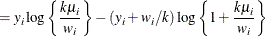
- Binomial
-


where
 and
and  are the events and trials in the events/trials syntax, and
  .
. ![$\mr {Var}[Y/n] = \mu (1-\mu )/n, \, \phi \equiv 1$](images/statug_glimmix0552.png) .
.
- Exponential
-
![\[ l(\mu _ i,\phi ;y_ i,w_ i) = \left\{ \begin{array}{ll} -\log \{ \mu _ i\} - y_ i/\mu _ i & w_ i = 1 \\ w_ i\log \left\{ \frac{w_ iy_ i}{\mu _ i}\right\} - \frac{w_ iy_ i}{\mu _ i} - \log \{ y_ i \Gamma (w_ i)\} & w_ i \not= 1 \end{array} \right. \]](images/statug_glimmix0553.png)
![$\mr {Var}[Y] = \mu ^2 , \, \phi \equiv 1$](images/statug_glimmix0554.png) .
.
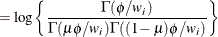
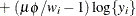
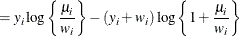
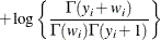
- Gamma
-
![\[ l(\mu _ i,\phi ;y_ i,w_ i) = w_ i\phi \log \left\{ \frac{w_ iy_ i\phi }{\mu _ i}\right\} - \frac{w_ iy_ i\phi }{\mu _ i} - \log \{ y_ i\} - \log \left\{ \Gamma (w_ i\phi )\right\} \]](images/statug_glimmix0555.png)
![$\mr {Var}[Y] = \phi \mu ^2, \, \phi > 0$](images/statug_glimmix0556.png) .
.
- Geometric
-
![$\mr {Var}[Y] = \mu + \mu ^2, \, \phi \equiv 1$](images/statug_glimmix0560.png) .
.
- Inverse Gaussian
-
![\[ l(\mu _ i,\phi ;y_ i,w_ i) = -\frac{1}{2} \left[ \frac{w_ i(y_ i-\mu _ i)^2}{y_ i\phi \mu _ i^2} + \log \left\{ \frac{\phi y_ i^3}{w_ i} \right\} + \log \{ 2\pi \} \right] \]](images/statug_glimmix0561.png)
![$\mr {Var}[Y] = \phi \mu ^3, \, \phi > 0$](images/statug_glimmix0562.png) .
.
- “Lognormal”
-
![\[ l(\mu _ i,\phi ;\log \{ y_ i\} ,w_ i) = -\frac{1}{2} \left[ \frac{w_ i(\log \{ y_ i\} -\mu _ i)^2}{\phi } + \log \left\{ \frac{\phi }{w_ i}\right\} + \log \{ 2\pi \} \right] \]](images/statug_glimmix0563.png)
![$\mr {Var}[\log \{ Y\} ] = \phi , \, \phi > 0$](images/statug_glimmix0564.png) .If you specify DIST=LOGNORMAL with response variable
.If you specify DIST=LOGNORMAL with response variable Y, the GLIMMIX procedure assumes that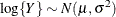 . Note that the preceding density is not the density of Y.
- Multinomial
-
![\[ l(\bmu _ i,\phi ;\mb {y}_ i,w_ i) = w_ i \sum _{j=1}^{J} y_{ij}\log \{ \mu _{ij}\} \]](images/statug_glimmix0565.png)
 .
.
- Negative Binomial
-
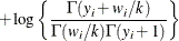
![$\mr {Var}[Y] = \mu + k\mu ^2, \, k > 0, \phi \equiv 1$](images/statug_glimmix0569.png) . For a given k, the negative binomial distribution is a member of the exponential family. The parameter k is related to the scale of the data, because it is part of the variance function. However, it cannot be factored from the
variance, as is the case with the
. For a given k, the negative binomial distribution is a member of the exponential family. The parameter k is related to the scale of the data, because it is part of the variance function. However, it cannot be factored from the
variance, as is the case with the  parameter in many other distributions. The parameter k is designated as “Scale” in the “Parameter Estimates” table of the GLIMMIX procedure.
- Normal (Gaussian)
-
![\[ l(\mu _ i,\phi ;y_ i,w_ i) = -\frac{1}{2} \left[ \frac{w_ i(y_ i-\mu _ i)^2}{\phi } + \log \left\{ \frac{\phi }{w_ i}\right\} + \log \{ 2\pi \} \right] \]](images/statug_glimmix0570.png)
![$\mr {Var}[Y] = \phi , \, \phi > 0$](images/statug_glimmix0571.png) .
.
- Poisson
-
![\[ l(\mu _ i,\phi ;y_ i,w_ i) = w_ i (y_ i \log \{ \mu _ i\} - \mu _ i - \log \{ \Gamma (y_ i + 1)\} ) \]](images/statug_glimmix0572.png)
![$\mr {Var}[Y] = \mu , \, \phi \equiv 1$](images/statug_glimmix0573.png) .
.
- Shifted T
-


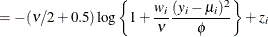
![$\phi > 0, \nu > 0, \, \mr {Var}[Y] = \phi \nu /(\nu -2)$](images/statug_glimmix0580.png) .
.
Define the parameter vector for the generalized linear model as ![]() , if
, if ![]() , and as
, and as ![]() otherwise.
otherwise. ![]() denotes the fixed-effects parameters in the linear predictor. For the negative binomial distribution, the relevant parameter
vector is
denotes the fixed-effects parameters in the linear predictor. For the negative binomial distribution, the relevant parameter
vector is ![]() . The gradient and Hessian of the negative log likelihood are then
. The gradient and Hessian of the negative log likelihood are then
The GLIMMIX procedure computes the gradient vector and Hessian matrix analytically, unless your programming statements involve
functions whose derivatives are determined by finite differences. If the procedure is in scoring mode, ![]() is replaced by its expected value. PROC GLIMMIX is in scoring mode when the number n of SCORING=n iterations has not been exceeded and the optimization technique uses second derivatives, or when the Hessian is computed
at convergence and the EXPHESSIAN option is in effect. Note that the objective function is the negative log likelihood when the GLIMMIX procedure fits a GLM
model. The procedure performs a minimization problem in this case.
is replaced by its expected value. PROC GLIMMIX is in scoring mode when the number n of SCORING=n iterations has not been exceeded and the optimization technique uses second derivatives, or when the Hessian is computed
at convergence and the EXPHESSIAN option is in effect. Note that the objective function is the negative log likelihood when the GLIMMIX procedure fits a GLM
model. The procedure performs a minimization problem in this case.
In models for independent data with known distribution, parameter estimates are obtained by the method of maximum likelihood. No parameters are profiled from the optimization. The default optimization technique for GLMs is the Newton-Raphson algorithm, except for Gaussian models with identity link, which do not require iterative model fitting. In the case of a Gaussian model, the scale parameter is estimated by restricted maximum likelihood, because this estimate is unbiased. The results from the GLIMMIX procedure agree with those from the GLM and REG procedure for such models. You can obtain the maximum likelihood estimate of the scale parameter with the NOREML option in the PROC GLIMMIX statement. To change the optimization algorithm, use the TECHNIQUE= option in the NLOPTIONS statement.
Standard errors of the parameter estimates are obtained from the inverse of the (observed or expected) second derivative matrix
![]() .
.