The CORRESP Procedure

In this example, PROC CORRESP reads an existing contingency table with supplementary observations and performs a simple correspondence analysis. The data are populations of the 50 U.S. states, grouped into regions, for each of the census years from 1920 to 1970 (U.S. Bureau of the Census, 1979). Alaska and Hawaii are treated as supplementary regions, because they were not states during this entire period and are not physically connected to the other 48 states. Consequently, it is reasonable to expect that population changes in these two states operate differently from population changes in the other states. The correspondence analysis is performed giving the supplementary points negative weight, and then the coordinates for the supplementary points are computed in the solution defined by the other points.
The initial DATA step reads the table, provides labels for the years, flags the supplementary rows with negative weights, and specifies absolute weights of 1000 for all observations since the data were originally reported in units of 1000 people.
In the PROC CORRESP statement, PRINT=PERCENT and the display options display the table of cell percentages (OBSERVED), cell contributions to the total chi-square scaled to sum to 100 (CELLCHI2), row profile rows that sum to 100 (RP), and column profile columns that sum to 100 (CP). The SHORT option specifies that the correspondence analysis summary statistics, contributions to inertia, and squared cosines should not be displayed. The option OUTC=COOR creates the output coordinate data set. Since the data are already in table form, a VAR statement is used to read the table. Row labels are specified with the ID statement, and column labels come from the variable labels. The WEIGHT statement flags the supplementary observations and restores the table values to populations.
The following statements produce Output 32.2.1:
title 'United States Population, 1920-1970';

data USPop;

   * Regions:
   * New England     - ME, NH, VT, MA, RI, CT.
   * Great Lakes     - OH, IN, IL, MI, WI.
   * South Atlantic  - DE, MD, DC, VA, WV, NC, SC, GA, FL.
   * Mountain        - MT, ID, WY, CO, NM, AZ, UT, NV.
   * Pacific         - WA, OR, CA.
   *
   * Note: Multiply data values by 1000 to get populations.;

   input Region $14. y1920 y1930 y1940 y1950 y1960 y1970;

   label y1920 = '1920'    y1930 = '1930'    y1940 = '1940'
         y1950 = '1950'    y1960 = '1960'    y1970 = '1970';

   if region = 'Hawaii' or region = 'Alaska'
      then w = -1000;       /* Flag Supplementary Observations */
      else w =  1000;

   datalines;
New England        7401  8166  8437  9314 10509 11842
NY, NJ, PA        22261 26261 27539 30146 34168 37199
Great Lakes       21476 25297 26626 30399 36225 40252
Midwest           12544 13297 13517 14061 15394 16319
South Atlantic    13990 15794 17823 21182 25972 30671
KY, TN, AL, MS     8893  9887 10778 11447 12050 12803
AR, LA, OK, TX    10242 12177 13065 14538 16951 19321
Mountain           3336  3702  4150  5075  6855  8282
Pacific            5567  8195  9733 14486 20339 25454
Alaska               55    59    73   129   226   300
Hawaii              256   368   423   500   633   769
;
ods graphics on;

* Perform Simple Correspondence Analysis;
proc corresp data=uspop print=percent observed cellchi2 rp cp
     short outc=Coor plot(flip);
   var y1920 -- y1970;
   id Region;
   weight w;
run;
The contingency table shows that the population of all regions increased over this time period. The row profiles show that population increased at a different rate for the different regions. There was a small increase in population in the Midwest, for example, but the population more than quadrupled in the Pacific region over the same period. The column profiles show that in 1920, the U.S. population was concentrated in the NY, NJ, PA, Great Lakes, Midwest, and South Atlantic regions. With time, the population shifted more to the South Atlantic, Mountain, and Pacific regions. This is also clear from the correspondence analysis. The inertia and chi-square decomposition table shows that there are five nontrivial dimensions in the table, but the association between the rows and columns is almost entirely one-dimensional.
Output 32.2.1: United States Population, 1920–1970
| United States Population, 1920-1970 |
| Contingency Table | |||||||
|---|---|---|---|---|---|---|---|
| Percents | 1920 | 1930 | 1940 | 1950 | 1960 | 1970 | Sum |
| New England | 0.830 | 0.916 | 0.946 | 1.045 | 1.179 | 1.328 | 6.245 |
| NY, NJ, PA | 2.497 | 2.946 | 3.089 | 3.382 | 3.833 | 4.173 | 19.921 |
| Great Lakes | 2.409 | 2.838 | 2.987 | 3.410 | 4.064 | 4.516 | 20.224 |
| Midwest | 1.407 | 1.492 | 1.516 | 1.577 | 1.727 | 1.831 | 9.550 |
| South Atlantic | 1.569 | 1.772 | 1.999 | 2.376 | 2.914 | 3.441 | 14.071 |
| KY, TN, AL, MS | 0.998 | 1.109 | 1.209 | 1.284 | 1.352 | 1.436 | 7.388 |
| AR, LA, OK, TX | 1.149 | 1.366 | 1.466 | 1.631 | 1.902 | 2.167 | 9.681 |
| Mountain | 0.374 | 0.415 | 0.466 | 0.569 | 0.769 | 0.929 | 3.523 |
| Pacific | 0.625 | 0.919 | 1.092 | 1.625 | 2.282 | 2.855 | 9.398 |
| Sum | 11.859 | 13.773 | 14.771 | 16.900 | 20.020 | 22.677 | 100.000 |
| Supplementary Rows | ||||||
|---|---|---|---|---|---|---|
| Percents | 1920 | 1930 | 1940 | 1950 | 1960 | 1970 |
| Alaska | 0.006170 | 0.006619 | 0.008189 | 0.014471 | 0.025353 | 0.033655 |
| Hawaii | 0.028719 | 0.041283 | 0.047453 | 0.056091 | 0.071011 | 0.086268 |
| Contributions to the Total Chi-Square Statistic | |||||||
|---|---|---|---|---|---|---|---|
| Percents | 1920 | 1930 | 1940 | 1950 | 1960 | 1970 | Sum |
| New England | 0.937 | 0.314 | 0.054 | 0.009 | 0.352 | 0.469 | 2.135 |
| NY, NJ, PA | 0.665 | 1.287 | 0.633 | 0.006 | 0.521 | 2.265 | 5.378 |
| Great Lakes | 0.004 | 0.085 | 0.000 | 0.001 | 0.005 | 0.094 | 0.189 |
| Midwest | 5.749 | 2.039 | 0.684 | 0.072 | 1.546 | 4.472 | 14.563 |
| South Atlantic | 0.509 | 1.231 | 0.259 | 0.000 | 0.285 | 1.688 | 3.973 |
| KY, TN, AL, MS | 1.454 | 0.711 | 1.098 | 0.087 | 0.946 | 2.945 | 7.242 |
| AR, LA, OK, TX | 0.000 | 0.069 | 0.077 | 0.001 | 0.059 | 0.030 | 0.238 |
| Mountain | 0.391 | 0.868 | 0.497 | 0.098 | 0.498 | 1.834 | 4.187 |
| Pacific | 18.591 | 9.380 | 5.458 | 0.074 | 7.346 | 21.248 | 62.096 |
| Sum | 28.302 | 15.986 | 8.761 | 0.349 | 11.558 | 35.046 | 100.000 |
| Row Profiles | ||||||
|---|---|---|---|---|---|---|
| Percents | 1920 | 1930 | 1940 | 1950 | 1960 | 1970 |
| New England | 13.2947 | 14.6688 | 15.1557 | 16.7310 | 18.8777 | 21.2722 |
| NY, NJ, PA | 12.5362 | 14.7888 | 15.5085 | 16.9766 | 19.2416 | 20.9484 |
| Great Lakes | 11.9129 | 14.0325 | 14.7697 | 16.8626 | 20.0943 | 22.3281 |
| Midwest | 14.7348 | 15.6193 | 15.8777 | 16.5167 | 18.0825 | 19.1691 |
| South Atlantic | 11.1535 | 12.5917 | 14.2093 | 16.8872 | 20.7060 | 24.4523 |
| KY, TN, AL, MS | 13.5033 | 15.0126 | 16.3655 | 17.3813 | 18.2969 | 19.4403 |
| AR, LA, OK, TX | 11.8687 | 14.1111 | 15.1401 | 16.8471 | 19.6433 | 22.3897 |
| Mountain | 10.6242 | 11.7898 | 13.2166 | 16.1624 | 21.8312 | 26.3758 |
| Pacific | 6.6453 | 9.7823 | 11.6182 | 17.2918 | 24.2784 | 30.3841 |
| Supplementary Row Profiles | ||||||
|---|---|---|---|---|---|---|
| Percents | 1920 | 1930 | 1940 | 1950 | 1960 | 1970 |
| Alaska | 6.5321 | 7.0071 | 8.6698 | 15.3207 | 26.8409 | 35.6295 |
| Hawaii | 8.6809 | 12.4788 | 14.3438 | 16.9549 | 21.4649 | 26.0766 |
| Column Profiles | ||||||
|---|---|---|---|---|---|---|
| Percents | 1920 | 1930 | 1940 | 1950 | 1960 | 1970 |
| New England | 7.0012 | 6.6511 | 6.4078 | 6.1826 | 5.8886 | 5.8582 |
| NY, NJ, PA | 21.0586 | 21.3894 | 20.9155 | 20.0109 | 19.1457 | 18.4023 |
| Great Lakes | 20.3160 | 20.6042 | 20.2221 | 20.1788 | 20.2983 | 19.9126 |
| Midwest | 11.8664 | 10.8303 | 10.2660 | 9.3337 | 8.6259 | 8.0730 |
| South Atlantic | 13.2343 | 12.8641 | 13.5363 | 14.0606 | 14.5532 | 15.1729 |
| KY, TN, AL, MS | 8.4126 | 8.0529 | 8.1857 | 7.5985 | 6.7521 | 6.3336 |
| AR, LA, OK, TX | 9.6888 | 9.9181 | 9.9227 | 9.6503 | 9.4983 | 9.5581 |
| Mountain | 3.1558 | 3.0152 | 3.1519 | 3.3688 | 3.8411 | 4.0971 |
| Pacific | 5.2663 | 6.6748 | 7.3921 | 9.6158 | 11.3968 | 12.5921 |
| United States Population, 1920-1970 |
| Inertia and Chi-Square Decomposition | |||||
|---|---|---|---|---|---|
| Singular Value |
Principal Inertia |
Chi- Square |
Percent |
Cumulative Percent |
20 40 60 80 100 ----+----+----+----+----+--- |
| 0.10664 | 0.01137 | 1.014E7 | 98.16 | 98.16 | ************************* |
| 0.01238 | 0.00015 | 136586 | 1.32 | 99.48 | |
| 0.00658 | 0.00004 | 38540 | 0.37 | 99.85 | |
| 0.00333 | 0.00001 | 9896.6 | 0.10 | 99.95 | |
| 0.00244 | 0.00001 | 5309.9 | 0.05 | 100.00 | |
| Total | 0.01159 | 1.033E7 | 100.00 | ||
| Degrees of Freedom = 40 | |||||
| Row Coordinates | ||
|---|---|---|
| Dim1 | Dim2 | |
| New England | 0.0611 | 0.0132 |
| NY, NJ, PA | 0.0546 | -0.0117 |
| Great Lakes | 0.0074 | -0.0028 |
| Midwest | 0.1315 | 0.0186 |
| South Atlantic | -0.0553 | 0.0105 |
| KY, TN, AL, MS | 0.1044 | -0.0144 |
| AR, LA, OK, TX | 0.0131 | -0.0067 |
| Mountain | -0.1121 | 0.0338 |
| Pacific | -0.2766 | -0.0070 |
| Supplementary Row Coordinates | ||
|---|---|---|
| Dim1 | Dim2 | |
| Alaska | -0.4152 | 0.0912 |
| Hawaii | -0.1198 | -0.0321 |
| Column Coordinates | ||
|---|---|---|
| Dim1 | Dim2 | |
| 1920 | 0.1642 | 0.0263 |
| 1930 | 0.1149 | -0.0089 |
| 1940 | 0.0816 | -0.0108 |
| 1950 | -0.0046 | -0.0125 |
| 1960 | -0.0815 | -0.0007 |
| 1970 | -0.1335 | 0.0086 |
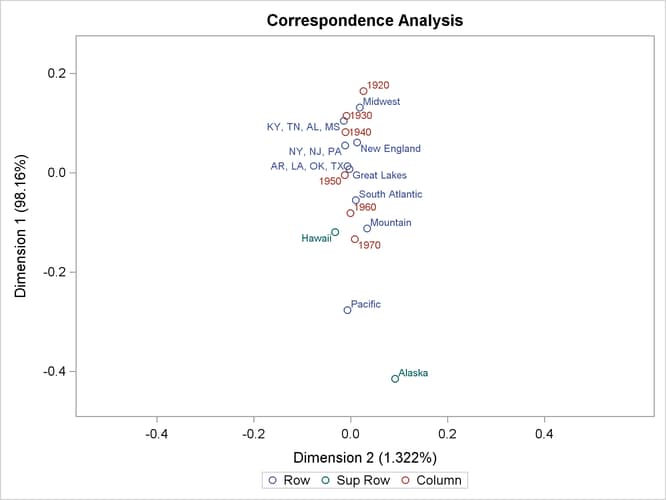
ODS Graphics is used to plot the results. The data are essentially one-dimensional. For data such as these, it is better to plot the first dimension vertically, as opposed to the default, which is horizontally. The vertical orientation has fewer opportunities for label collisions. Specifying PLOTS(FLIP) on the PROC CORRESP statement switches the vertical and horizontal axes to improve the graphical display.
The plot shows that the first dimension correctly orders the years. There is nothing in the correspondence analysis that forces this to happen; the analysis has no information about the inherent ordering of the column categories. The ordering of the regions and the ordering of the years reflect the shift over time of the U.S. population from the Northeast quadrant of the country to the South and to the West. The results show that the West and Southeast grew faster than the rest of the contiguous 48 states during this period.
The plot also shows that the growth pattern for Hawaii was similar to the growth pattern for the mountain states and that Alaska’s growth was even more extreme than the Pacific states’ growth. The row profiles confirm this interpretation.
The Pacific region is farther from the origin than all other active points. The Midwest is the extreme region in the other direction. The table of contributions to the total chi-square shows that 62% of the total chi-square statistic is contributed by the Pacific region, which is followed by the Midwest at over 14%. Similarly the two extreme years, 1920 and 1970, together contribute over 63% to the total chi-square, whereas the years nearer the origin of the plot contribute less.