The SURVEYMEANS Procedure

Geometric Mean
For a continuous variable Y that has positive values, the SURVEYMEANS procedure can compute its geometric mean and associated standard error and confidence
limits. To request these statistics, you can specify statistic-keywords such as GEOMEAN, GEOSTDERR, and GEOMLCLM.
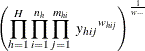
The geometric mean of Y from a sample is computed as
|
|
|
 |
|
|
|
|
where
|
|
is the sum of the weights over all observations in the data set.
When you use the Taylor series method, the variance estimation for the geometric mean is computed as
|
|
|
|
where
|
|
|
|
|
|
|
|
The standard error of the geometric mean is the square root of the estimated variance:
|
|
The confidence limits for the geometric means are computed based on the confidence limits for the log transformation of the
Y variable as
|
|
where
|
|
and ![]() is the
is the ![]() percentile of the t distribution, with df calculated as in the section t Test for the Mean.
percentile of the t distribution, with df calculated as in the section t Test for the Mean.
If you use replication methods to estimate the variance by specifying VARMETHOD=BRR or VARMETHOD=JACKKNIFE, the procedure computes the variance of a geometric means ![]() by using the variability among replicate estimates to estimate the overall variance. See the section Replication Methods for Variance Estimation for more information.
by using the variability among replicate estimates to estimate the overall variance. See the section Replication Methods for Variance Estimation for more information.
Then the standard error is the square root of the estimated variance:
|
|
The confidence limits for the geometric means are computed based on the confidence limits for the log transformation of the
variable Y as
|
|
where
|
|
and ![]() is the
is the ![]() percentile of the t distribution, with df calculated as in the section t Test for the Mean.
percentile of the t distribution, with df calculated as in the section t Test for the Mean.