The RSREG Procedure

A Response Surface with a Simple Optimum
This example uses the three-factor quadratic model discussed in John (1971). Settings of the temperature, gas–liquid ratio, and packing height are controlled factors in the production of a certain
chemical; Schneider and Stockett (1963) performed an experiment in order to determine the values of these three factors that minimize the unpleasant odor of the
chemical. The following statements input the SAS data set smell; the variable Odor is the response, while the variables T, R, and H are the independent factors.
title 'Response Surface with a Simple Optimum';
data smell;
   input Odor T R H @@;
   label
      T = "Temperature"
      R = "Gas-Liquid Ratio"
      H = "Packing Height";
   datalines;
 66 40 .3 4     39 120 .3 4     43 40 .7 4     49 120 .7  4
 58 40 .5 2     17 120 .5 2     -5 40 .5 6    -40 120 .5  6
 65 80 .3 2      7  80 .7 2     43 80 .3 6    -22  80 .7  6
-31 80 .5 4    -35  80 .5 4    -26 80 .5 4
;
The following statements invoke PROC RSREG on the data set smell. Figure 81.1 through Figure 81.3 display the results of the analysis, including a lack-of-fit test requested with the LACKFIT option.
proc rsreg data=smell;
   model Odor = T R H / lackfit;
run;
Figure 81.1 displays the coding coefficients for the transformation of the independent variables to lie between –1 and 1, simple statistics for the response variable, hypothesis tests for linear, quadratic, and crossproduct terms, and the lack-of-fit test. The hypothesis tests can be used to gain a rough idea of importance of the effects; here the crossproduct terms are not significant. However, the lack of fit for the model is significant, so more complicated modeling or further experimentation with additional variables should be performed before firm conclusions are made concerning the underlying process.
Figure 81.1: Summary Statistics and Analysis of Variance
| Response Surface with a Simple Optimum |
| Coding Coefficients for the Independent Variables |
||
|---|---|---|
| Factor | Subtracted off | Divided by |
| T | 80.000000 | 40.000000 |
| R | 0.500000 | 0.200000 |
| H | 4.000000 | 2.000000 |
| Response Surface for Variable Odor | |
|---|---|
| Response Mean | 15.200000 |
| Root MSE | 22.478508 |
| R-Square | 0.8820 |
| Coefficient of Variation | 147.8849 |
| Regression | DF | Type I Sum of Squares | R-Square | F Value | Pr > F |
|---|---|---|---|---|---|
| Linear | 3 | 7143.250000 | 0.3337 | 4.71 | 0.0641 |
| Quadratic | 3 | 11445 | 0.5346 | 7.55 | 0.0264 |
| Crossproduct | 3 | 293.500000 | 0.0137 | 0.19 | 0.8965 |
| Total Model | 9 | 18882 | 0.8820 | 4.15 | 0.0657 |
| Residual | DF | Sum of Squares | Mean Square | F Value | Pr > F |
|---|---|---|---|---|---|
| Lack of Fit | 3 | 2485.750000 | 828.583333 | 40.75 | 0.0240 |
| Pure Error | 2 | 40.666667 | 20.333333 | ||
| Total Error | 5 | 2526.416667 | 505.283333 |
Parameter estimates and the factor ANOVA are shown in Figure 81.2. Looking at the parameter estimates, you can see that the crossproduct terms are not significantly different from zero, as
noted previously. The Estimate column contains estimates based on the raw data, and the Parameter Estimate from Coded Data
column contains estimates based on the coded data. The factor ANOVA table displays tests for all four parameters corresponding
to each factor—the parameters corresponding to the linear effect, the quadratic effect, and the effects of the crossproducts
with each of the other two factors. The only factor with a significant overall effect is R, indicating that the level of noise left unexplained by the model is still too high to estimate the effects of T and H accurately. This might be due to the lack of fit.
Figure 81.2: Parameter Estimates and Hypothesis Tests
| Parameter | DF | Estimate | Standard Error | t Value | Pr > |t| | Parameter Estimate from Coded Data |
|---|---|---|---|---|---|---|
| Intercept | 1 | 568.958333 | 134.609816 | 4.23 | 0.0083 | -30.666667 |
| T | 1 | -4.102083 | 1.489024 | -2.75 | 0.0401 | -12.125000 |
| R | 1 | -1345.833333 | 335.220685 | -4.01 | 0.0102 | -17.000000 |
| H | 1 | -22.166667 | 29.780489 | -0.74 | 0.4902 | -21.375000 |
| T*T | 1 | 0.020052 | 0.007311 | 2.74 | 0.0407 | 32.083333 |
| R*T | 1 | 1.031250 | 1.404907 | 0.73 | 0.4959 | 8.250000 |
| R*R | 1 | 1195.833333 | 292.454665 | 4.09 | 0.0095 | 47.833333 |
| H*T | 1 | 0.018750 | 0.140491 | 0.13 | 0.8990 | 1.500000 |
| H*R | 1 | -4.375000 | 28.098135 | -0.16 | 0.8824 | -1.750000 |
| H*H | 1 | 1.520833 | 2.924547 | 0.52 | 0.6252 | 6.083333 |
| Factor | DF | Sum of Squares | Mean Square | F Value | Pr > F | Label |
|---|---|---|---|---|---|---|
| T | 4 | 5258.016026 | 1314.504006 | 2.60 | 0.1613 | Temperature |
| R | 4 | 11045 | 2761.150641 | 5.46 | 0.0454 | Gas-Liquid Ratio |
| H | 4 | 3813.016026 | 953.254006 | 1.89 | 0.2510 | Packing Height |
Figure 81.3 displays the canonical analysis and eigenvectors. The canonical analysis indicates that the directions of principal orientation
for the predicted response surface are along the axes associated with the three factors, confirming the small interaction
effect in the regression ANOVA (Figure 81.1). The largest eigenvalue (48.8588) corresponds to the eigenvector (0.238091, 0.971116, -0.015690), the largest component
of which (0.971116) is associated with R; similarly, the second-largest eigenvalue (31.1035) is associated with T. The third eigenvalue (6.0377), associated with H, is quite a bit smaller than the other two, indicating that the response surface is relatively insensitive to changes in
this factor. The coded form of the canonical analysis indicates that the estimated response surface is at a minimum when T and R are both near the middle of their respective ranges (that is, the coded critical values for T and R are both near 0) and H is relatively high; in uncoded terms, the model predicts that the unpleasant odor is minimized when T = 84.876502, R = 0.539915, and H = 7.541050.
Figure 81.3: Canonical Analysis and Eigenvectors
| Factor | Critical Value | Label | |
|---|---|---|---|
| Coded | Uncoded | ||
| T | 0.121913 | 84.876502 | Temperature |
| R | 0.199575 | 0.539915 | Gas-Liquid Ratio |
| H | 1.770525 | 7.541050 | Packing Height |
| Predicted value at stationary point: -52.024631 | |||
| Eigenvalues | Eigenvectors | ||
|---|---|---|---|
| T | R | H | |
| 48.858807 | 0.238091 | 0.971116 | -0.015690 |
| 31.103461 | 0.970696 | -0.237384 | 0.037399 |
| 6.037732 | -0.032594 | 0.024135 | 0.999177 |
| Stationary point is a minimum. | |||
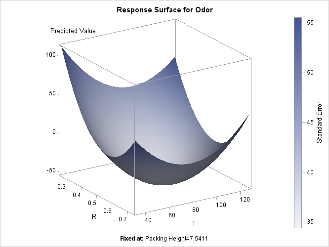
To plot the response surface with respect to two of the factor variables, fix H, the least significant factor variable, at its estimated optimum value. The following statements use ODS Graphics to display
the surface:
ods graphics on;
proc rsreg data=smell
           plots(unpack)=surface(3d at(H=7.541050));
   model Odor = T R H;
   ods select 'T * R = Pred';
run;
ods graphics off;
Note that the ODS SELECT statement is specified to select the plot of interest.
Figure 81.4: The Response Surface at the Optimum H
Alternatively, the following statements produce an output data set containing the surface information, which you can then
use for plotting surfaces or searching for optima. The first DATA step fixes H, the least significant factor variable, at its estimated optimum value (7.541), and generates a grid of points for T and R. To ensure that the grid data do not affect parameter estimates, the response variable (Odor) is set to missing. (See the section Missing Values.) The second DATA step concatenates these grid points to the original data. Then PROC RSREG computes predictions for the
combined data. The last DATA step subsets the predicted values over just the grid points, which excludes the predictions at
the original data.
data grid;
   do;
      Odor =  .  ;
      H    = 7.541;
      do T = 20 to 140 by 5;
         do R = .1 to .9 by .05;
            output;
         end;
      end;
   end;
run;
data grid;
   set smell grid;
run;

proc rsreg data=grid out=predict noprint;
   model Odor = T R H / predict;
run;

data grid;
   set predict;
   if H = 7.541;
run;