The PRINCOMP Procedure

Example 73.1 Temperatures
This example analyzes mean daily temperatures in selected cities in January and July. Both the raw data and the principal components are plotted to illustrate how principal components are orthogonal rotations of the original variables.
The following statements create the Temperature data set.
data Temperature;
   length Cityid $ 2;
   title 'Mean Temperature in January and July for Selected Cities ';
   input City $1-15 January July;
   Cityid = substr(City,1,2);
   datalines;
Mobile          51.2 81.6
Phoenix         51.2 91.2
Little Rock     39.5 81.4
Sacramento      45.1 75.2
Denver          29.9 73.0

   ... more lines ...

Cheyenne        26.6 69.1
;
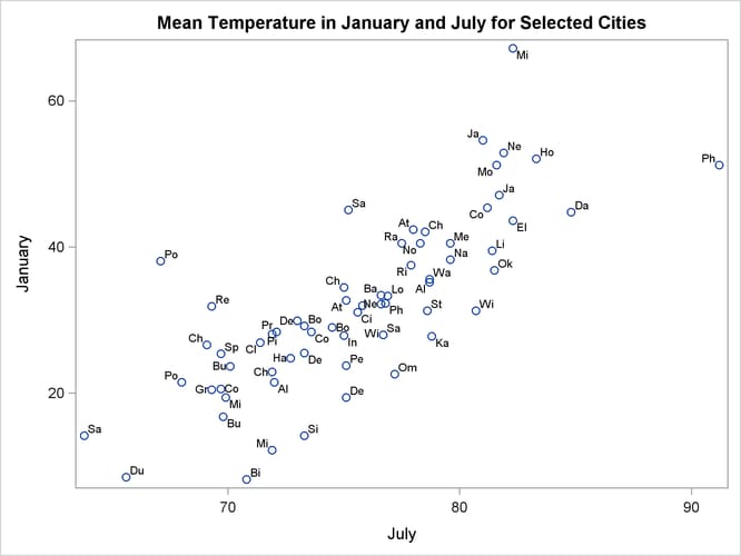
The following statements plot the temperature data set. The Cityid variable instead of City is used as a data label in the scatter plot for possible label clashing.
title 'Mean Temperature in January and July for Selected Cities';
proc sgplot data=Temperature;
   scatter x=July y=January / datalabel=Cityid;
run;
The results are displayed in Output 73.1.1, which shows a scatter diagram of the 64 pairs of data points with July temperatures plotted against January temperatures.
Output 73.1.1: Plot of Raw Data
The following step requests a principal component analysis on the Temperature data set:
ods graphics on;

title 'Mean Temperature in January and July for Selected Cities';
proc princomp data=Temperature cov plots=score(ellipse);
   var July January;
   id Cityid;
run;
Output 73.1.2 displays the PROC PRINCOMP output. The standard deviation of January (11.712) is higher than the standard deviation of July (5.128). The COV option in the PROC PRINCOMP statement requests the principal components to be computed from the covariance
matrix. The total variance is 163.474. The first principal component explains about 94% of the total variance, and the second
principal component explains only about 6%. The eigenvalues sum to the total variance.
Note that January receives a higher loading on Prin1 because it has a higher standard deviation than July, and the PRINCOMP procedure calculates the scores by using the centered variables rather than the standardized variables.
Output 73.1.2: Results of Principal Component Analysis
| Mean Temperature in January and July for Selected Cities |
| Observations | 64 |
|---|---|
| Variables | 2 |
| Simple Statistics | ||
|---|---|---|
| July | January | |
| Mean | 75.60781250 | 32.09531250 |
| StD | 5.12761910 | 11.71243309 |
| Covariance Matrix | ||
|---|---|---|
| July | January | |
| July | 26.2924777 | 46.8282912 |
| January | 46.8282912 | 137.1810888 |
| Total Variance | 163.47356647 |
|---|
| Eigenvalues of the Covariance Matrix | ||||
|---|---|---|---|---|
| Eigenvalue | Difference | Proportion | Cumulative | |
| 1 | 154.310607 | 145.147647 | 0.9439 | 0.9439 |
| 2 | 9.162960 | 0.0561 | 1.0000 | |
| Eigenvectors | ||
|---|---|---|
| Prin1 | Prin2 | |
| July | 0.343532 | 0.939141 |
| January | 0.939141 | -.343532 |
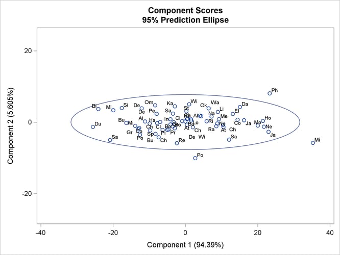
PLOTS=SCORE in the PROC PRINCOMP statement requests a plot of the second principal component against the first principal component
as shown in Output 73.1.3. It is clear from this plot that the principal components are orthogonal rotations of the original variables and that the
first principal component has a larger variance than the second principal component. In fact, the first component has a larger
variance than either of the original variables July and January. The ellipse indicates that Miami, Phoenix, and Portland are possible outliers.
Output 73.1.3: Plot of Component 2 by Component 1