The MDS Procedure

Getting Started: MDS Procedure
The simplest application of PROC MDS is to reconstruct a map from a table of distances between points on the map (Kruskal
and Wish 1978, pp. 7–9). A data set containing a table of flying mileages between 10 U.S. cities is available in the Sashelp library.
Since the flying mileages are very good approximations to Euclidean distance, no transformation is needed to convert distances from the model to data. The analysis can therefore be done at the absolute level of measurement, as displayed in the following PROC MDS step (LEVEL=ABSOLUTE). The following statements produce Figure 56.1 and Figure 56.2:
title 'Analysis of Flying Mileages between Ten U.S. Cities';

ods graphics on;

proc mds data=sashelp.mileages level=absolute;
   id city;
run;
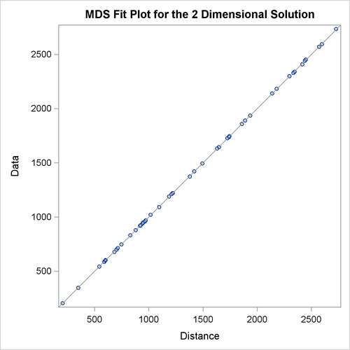
PROC MDS first displays the iteration history. In this example, only one iteration is required. The badness-of-fit criterion 0.001689 indicates that the data fit the model extremely well. You can also see that the fit is excellent in the fit plot in Figure 56.2.
Figure 56.1: Iteration History from PROC MDS
| Analysis of Flying Mileages between Ten U.S. Cities |
| Iteration | Type | Badness- of-Fit Criterion |
Change in Criterion |
Convergence Measure |
|---|---|---|---|---|
| 0 | Initial | 0.003273 | . | 0.8562 |
| 1 | Lev-Mar | 0.001689 | 0.001584 | 0.005128 |
| Convergence criterion is satisfied. |
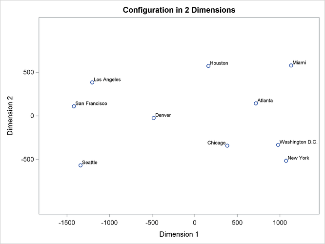
While PROC MDS can recover the relative positions of the cities, it cannot determine absolute location or orientation. In this case, north is toward the bottom of the plot. (See the first plot in Figure 56.2.)
Figure 56.2: Plot of Estimated Configuration and Fit