The LIFETEST Procedure

Example 52.2 Enhanced Survival Plot and Multiple-Comparison Adjustments
This example highlights a number of features in the survival plot that uses ODS Graphics. Also shown in this example are
comparisons of survival curves based on multiple comparison adjustments. Data of 137 bone marrow transplant patients extracted
from Klein and Moeschberger (1997) have been saved in the data set BMT in the Sashelp library. At the time of transplant, each patient is classified into one of three risk categories: ALL (acute lymphoblastic
leukemia), AML (acute myelocytic leukemia)-Low Risk, and AML-High Risk. The endpoint of interest is the disease-free survival
time, which is the time to death or relapse or to the end of the study in days. In this data set, the variable Group represents the patient’s risk category, the variable T represents the disease-free survival time, and the variable Status is the censoring indicator, with the value 1 indicating an event time and the value 0 a censored time.
The following step displays the first 10 observations of the BMT data set in Output 52.2.1. The data set is available in the Sashelp library.
proc print data=Sashelp.BMT(obs=10);
run;
Output 52.2.1: A Subset of the Bone Marrow Transplant Data
| Obs | Group | T | Status |
|---|---|---|---|
| 1 | ALL | 2081 | 0 |
| 2 | ALL | 1602 | 0 |
| 3 | ALL | 1496 | 0 |
| 4 | ALL | 1462 | 0 |
| 5 | ALL | 1433 | 0 |
| 6 | ALL | 1377 | 0 |
| 7 | ALL | 1330 | 0 |
| 8 | ALL | 996 | 0 |
| 9 | ALL | 226 | 0 |
| 10 | ALL | 1199 | 0 |
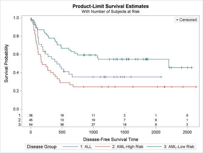
In the following statements, PROC LIFETEST is invoked to compute the product-limit estimate of the survivor function for each risk category. Using ODS Graphics, you can display the number of subjects at risk in the survival plot. The PLOTS= option requests that the survival curves be plotted, and the ATRISK= suboption specifies the time points at which the at-risk numbers are displayed. In the STRATA statement, the ADJUST=SIDAK option requests the Šidák multiple-comparison adjustment, and by default, all paired comparisons are carried out.
ods graphics on;

proc lifetest data=sashelp.BMT plots=survival(atrisk=0 to 2500 by 500);
   time T * Status(0);
   strata Group / test=logrank adjust=sidak;
run;
Output 52.2.2 displays the estimated disease-free survival for the three leukemia groups with the number of subjects at risk at 0, 500, 1,000, 1,500, 2,000, and 2,500 days. Patients in the AML-Low Risk group experience a longer disease-free survival than those in the ALL group, who in turn fare better than those in the AML-High Risk group.
Output 52.2.2: Estimated Disease-Free Survival for 137 Bone Marrow Transplant Patients
The log-rank test (Output 52.2.3) shows that the disease-free survival times for these three risk groups are significantly different (p = 0.001).
Output 52.2.3: Log-Rank Test of Disease Group Homogeneity
| Test of Equality over Strata | |||
|---|---|---|---|
| Test | Chi-Square | DF | Pr > Chi-Square |
| Log-Rank | 13.8037 | 2 | 0.0010 |
The Šidák multiple-comparison results are shown in Output 52.2.4. There is no significant difference in disease-free survivor functions between the ALL and AML-High Risk groups (p = 0.2779). The difference between the ALL and AML-Low Risk groups is marginal (p = 0.0685), but the AML-Low Risk and AML-High Risk groups have significantly different disease-free survivor functions (p = 0.0006).
Output 52.2.4: All Paired Comparsions
| Adjustment for Multiple Comparisons for the Logrank Test | ||||
|---|---|---|---|---|
| Strata Comparison | Chi-Square | p-Values | ||
| Group | Group | Raw | Sidak | |
| ALL | AML-High Risk | 2.6610 | 0.1028 | 0.2779 |
| ALL | AML-Low Risk | 5.1400 | 0.0234 | 0.0685 |
| AML-High Risk | AML-Low Risk | 13.8011 | 0.0002 | 0.0006 |
Suppose you consider the AML-Low Risk group as the reference group. You can use the DIFF= option in the STRATA statement to designate this risk group as the control and apply a multiple-comparison adjustment to the p-values for the paired comparison between the AML-Low Risk group with each of the other groups. Consider the Šidák correction again. You specify the ADJUST= and DIFF= options as in the following statements:
proc lifetest data=sashelp.BMT notable plots=none;
   time T * Status(0);
   strata Group / test=logrank adjust=sidak diff=control('AML-Low Risk');
run;
Output 52.2.5 shows that although both the ALL and AML-High Risk groups differ from the AML-Low Risk group at the 0.05 level, the difference between the AML-High Risk and the AML-Low Risk group is highly significant (p = 0.0004).
Output 52.2.5: Comparisons with the Reference Group
| Adjustment for Multiple Comparisons for the Logrank Test | ||||
|---|---|---|---|---|
| Strata Comparison | Chi-Square | p-Values | ||
| Group | Group | Raw | Sidak | |
| ALL | AML-Low Risk | 5.1400 | 0.0234 | 0.0462 |
| AML-High Risk | AML-Low Risk | 13.8011 | 0.0002 | 0.0004 |
The survival plot that is displayed in Output 52.2.2 might be sufficient for many purposes, but you might have other preferences. Typical alternatives include displaying the
number of subjects at risk outside the plot area, reordering the stratum labels in the survival plot legend, and displaying
the strata in the at-risk table by using their full labels. PROC LIFETEST provides options that you can use to make these
changes without requiring template changes. In the sashelp.BMT data set, the variable Group that represents the strata is a character variable with three values, namely (in alphabetical order), ALL, AML-High Risk,
and AML-Low Risk. It might be desirable to present the strata in the order ALL, AML-Low Risk, and AML-High Risk. The ORDER=INTERNAL
option in the STRATA statement enables you to order the strata by their internal values. In the following statements, the
new dataset Bmt2 is a copy of sashelp.BMT with the variable Group changed to a a numeric variable with values 1, 2, and 3 representing ALL, AML-Low Risk, and AML-High Risk, respectively.
The original character values of Group are kept as the formatted values, which are used to label the strata in the printed output.
proc format;
   invalue $bmtifmt 'ALL' = 1 'AML-Low Risk' = 2 'AML-High Risk' = 3;
   value bmtfmt 1 = 'ALL'  2 = 'AML-Low Risk' 3 = 'AML-High Risk';
run;

data Bmt2;
   set sashelp.BMT(rename=(Group=G));
   Group = input(input(G, $bmtifmt.), 1.);
   label Group = 'Disease Group';
   format Group bmtfmt.;
   run;
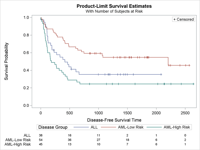
The following statements produce a survival plot that has all the aforementioned modifications. The new data set Bmt2 is used as the input data. The OUTSIDE and MAXLEN= options are specified in the PLOTS= option. The OUTSIDE option draws the
at-risk table outside the plot area. Because the longest label of the strata has 13 characters, specifying MAXLEN=13 is sufficient
to display all the stratum labels in the at-risk table. The ORDER=INTERNAL option in the STRATA statement orders the strata
by their numerical values 1, 2, and 3, which represent the order ALL, AML-Low Risk, and AML-High Risk, respectively.
proc LIFETEST data=Bmt2 plots=s(atrisk(outside maxlen=13)=0 to 2500 by 500);
   time T*Status(0);
   strata Group / order=internal;
run;
The modified survival plot is displayed in Output 52.2.6. The most noticeable change from Output 52.2.2 is that the number of subjects at risk is displayed below the time axis. Other changes include displaying the full labels of the strata in the at-risk table and presenting the strata in the order ALL, AML-Low Risk, and AML-High Risk.
Output 52.2.6: Modified Disease-Free Survival for Bone Marrow Transplant Patients
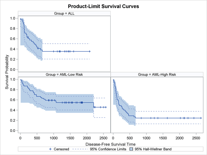
Klein and Moeschberger (1997, Section 4.4) describe in detail how to compute the Hall-Wellner (HW) and equal-precision (EP) confidence bands for the survivor function. You can output these simultaneous confidence intervals to a SAS data set by using the CONFBAND= and OUTSURV= options in the PROC LIFETEST statement. You can display survival curves with pointwise and simultaneous confidence limits through ODS Graphics. When the survival data are stratified, displaying all the survival curves and their confidence limits in the same plot can make the plot appear cluttered. In the following statements, the PLOTS= specification requests that the survivor functions be displayed along with their pointwise confidence limits (CL) and Hall-Wellner confidence bands (CB=HW). The STRATA=PANEL specification requests that the survival curves be displayed in a panel of three plots, one for each risk group.
proc lifetest data=Bmt2 plots=survival(cl cb=hw strata=panel);
   time T * Status(0);
   strata Group/order=internal;
run;

ods graphics off;
The panel plot is shown in Output 52.2.7.
Output 52.2.7: Estimated Disease-Free Survivor Functions with Confidence Limits