Example 19.3 Logistic Regression
Consider a study of the analgesic effects of treatments on elderly patients with neuralgia. Two test treatments and a placebo
are compared. The response variable is whether the patient reported pain or not. Researchers recorded the age and gender of
60 patients and the duration of complaint before the treatment began. The following DATA step creates the data set Neuralgia:
data Neuralgia;
   input Treatment $ Sex $ Age Duration Pain $ @@;
   datalines;
P  F  68   1  No   B  M  74  16  No  P  F  67  30  No
P  M  66  26  Yes  B  F  67  28  No  B  F  77  16  No
A  F  71  12  No   B  F  72  50  No  B  F  76   9  Yes
A  M  71  17  Yes  A  F  63  27  No  A  F  69  18  Yes
B  F  66  12  No   A  M  62  42  No  P  F  64   1  Yes
A  F  64  17  No   P  M  74   4  No  A  F  72  25  No
P  M  70   1  Yes  B  M  66  19  No  B  M  59  29  No
A  F  64  30  No   A  M  70  28  No  A  M  69   1  No
B  F  78   1  No   P  M  83   1  Yes B  F  69  42  No
B  M  75  30  Yes  P  M  77  29  Yes P  F  79  20  Yes
A  M  70  12  No   A  F  69  12  No  B  F  65  14  No
B  M  70   1  No   B  M  67  23  No  A  M  76  25  Yes
P  M  78  12  Yes  B  M  77   1  Yes B  F  69  24  No
P  M  66   4  Yes  P  F  65  29  No  P  M  60  26  Yes
A  M  78  15  Yes  B  M  75  21  Yes A  F  67  11  No
P  F  72  27  No   P  F  70  13  Yes A  M  75   6  Yes
B  F  65   7  No   P  F  68  27  Yes P  M  68  11  Yes
P  M  67  17  Yes  B  M  70  22  No  A  M  65  15  No
P  F  67   1  Yes  A  M  67  10  No  P  F  72  11  Yes
A  F  74   1  No   B  M  80  21  Yes A  F  69   3  No
;
The Neuralgia data set contains five variables. The Pain variable is the response. A specification of Pain=Yes indicates that the patient felt pain, and Pain=No indicates that the patient did not feel pain. The variable Treatment is a categorical variable with three levels: A and B represent the two test treatments, and P represents the placebo treatment.
The gender of the patients is given by the categorical variable Sex. The variable Age is the age of the patients, in years, when treatment began. The duration of complaint, in months, before the treatment began
is given by the variable Duration.
In the following statements, a complex model that includes classification and continuous covariates and an interaction term
is fit to the Neuralgia data. When you try to create a default effect plot from this model, computations stop because the best type of plot cannot
easily be determined.
ods graphics on;
proc logistic data=Neuralgia;
   class Treatment Sex / param=ref;
   model Pain= Treatment|Sex Age Duration;
   effectplot;
run;
ods graphics off;
To produce an effect plot for this model, you need to first choose the type of plot to be created. In this case, since there
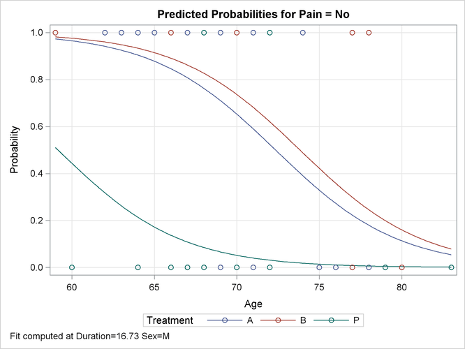
are both classification and continuous covariates on the model, a SLICEFIT plot-type displays the first continuous covariate (Age) on the X axis and displays fit curves that correspond to each level of the first classification covariate (Treatment). The following statements produce Output 19.3.1.
ods graphics on;
proc logistic data=Neuralgia;
   class Treatment Sex / param=ref;
   model Pain= Treatment|Sex Age Duration;
   effectplot slicefit;
run;
ods graphics off;
By default, effect plots from PROC LOGISTIC are displayed on the probability scale. The predicted values are computed at the
mean of the Duration variable, 16.73, and at the reference level of the Sex variable, M. Observations are also displayed on the sliced-fit plot in Output 19.3.1. While the display of binary responses can give you a feel for the spread of the data, it does not enable you to evaluate
the fit of the model.
Output 19.3.1: Default Fit Plot Sliced by Treatment
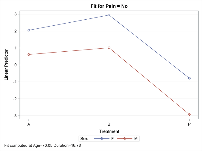
In the following statements, an INTERACTION plot-type is specified for the Treatment variable, with the Sex effect chosen for grouping the fits. The Age and Duration variables are set to their mean values for computing the predicted values. The NOOBS option suppresses the display of the binary observations on this plot. The LINK option is specified to display the fit on the LOGIT scale; if there is no interaction between Treatment and Sex, then the resulting curves shown in Output 19.3.2 will have similar slopes across the treatments.
ods graphics on;
proc logistic data=Neuralgia;
   class Treatment Sex / param=ref;
   model Pain= Treatment|Sex Age Duration;
   effectplot interaction(x=Treatment sliceby=Sex) / noobs link;
run;
ods graphics off;
In Output 19.3.2, the slopes of the lines seem “parallel” across the treatments, corroborating the nonsignificance of the interaction terms.
Output 19.3.2: Interaction Plot of an Interaction Effect
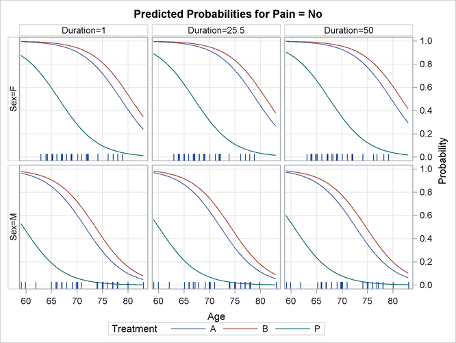
In the following statements, the interaction effect is removed, and the Duration variable is investigated further. The PLOTBY(ROWS)= option displays the Sex levels in the rows of a panel of plots, and the AT option computes the fits for several values of the Duration main effect in the columns of the panel. The OBS(FRINGE) option moves the observations to a fringe (rug) plot at the bottom of the plot, the observations are subsetted and displayed
according to the value of the PLOTBY= variable, and the JITTER option makes overlaid fringes more visible. A STORE statement is also specified to save the model information for a later display. These statements produce Output 19.3.3.
ods graphics on;
proc logistic data=Neuralgia;
   class Treatment Sex / param=ref;
   model Pain= Treatment Sex Age Duration;
   effectplot slicefit(sliceby=Treatment plotby(rows)=Sex)
      / at(Duration=min midrange max) obs(fringe jitter(seed=39393));
   store logimodel;
run;
ods graphics off;
The predicted probability curves in Output 19.3.3 look very similar across the different values of the Duration variable, which agrees with the nonsignificance of Duration in this model. The fringe plot displays only female patients in the SEX=F row of the panel and displays only male patients
in the SEX=M row, because the PLOTBY=SEX option subsets the observations.
Output 19.3.3: Sliced-Fit Plot with AT Option
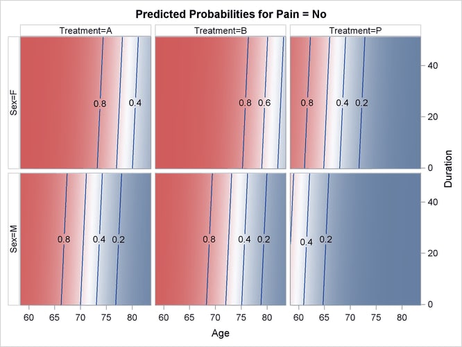
The following statements use the stored model and the PLM procedure to display a panel of contour plots:
ods graphics on;
proc plm restore=logimodel;
   effectplot contour(plotby=Treatment) / at(Sex=all);
run;
ods graphics off;
Output 19.3.4 again confirms that Duration is not significant.
Output 19.3.4: Contour Fit Panel